Chapter 9: Energy storage II

Chapter overview

This chapter extends the model in Chapter 8 by starting with a more complex energy storage problem that combines energy from two sources (a wind farm and the grid) to serve a time-dependent load, helped by a storage device. A distinguishing feature of this problem is that we are given a 24-hour forecast of wind which is updated every hour. These forecasts can change quite a bit over time, so this introduces a new source of uncertainty, which is not just that the forecasts are not perfect, but that the forecasts themselves are changing.

We start by exploring two models for modeling the uncertainty in the forecasts of wind. The first is a method known as Gaussian process regression, which is useful for modeling continuous processes such as the amount of wind energy that we expect to be generated over the next 24 hours.

The second method uses a powerful, yet surprisingly simple, method based on what are called “hidden state models” that allow us to replicate a property of forecasts known as crossing times. These refer to the amount of time that a forecast is above, or below, the actual. This is an important behavior when modeling storage problems.

To design our policy we adapt the technique that we first introduced in Chapter 6, where we started with a deterministic lookahead policy, and then introduced parameters to help it work better over time. For our energy problem, we plan using our best estimate of the forecasted energy from wind multiplied by coefficients that depend on how many hours we are forecasting into the future. This gives us a deterministic optimization model with 24 parameters that have to be tuned.

Narrative

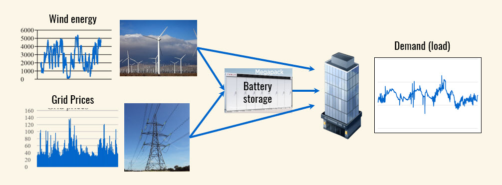
We are now going to solve a somewhat more complex energy storage problem depicted in Figure 9.1. In contrast with our previous storage system that just bought and sold energy from the grid, we now face the problem of meeting a time-dependent load for a building using energy from a wind farm and the grid, with a single energy storage device to help smooth the different processes.

This problem is also going to exhibit another distinctive property, which is that all the exogenous processes (wind, prices, loads and temperature) are going to come from a dynamic process that varies with different types of predictability:

• Loads – The load (which is the demand for energy) follows a fairly predictable pattern that depends on time of day (a building needs to be at a particular temperature by 8am when people start showing up) as well as temperature.
• Temperature – The temperature is a reasonably predictable process that depends on time of day and season, but also reflects local weather conditions that can be forecasted with some accuracy.
• Wind – There are vendors who perform forecasting services for wind, although the forecasts are not very accurate and evolve fairly quickly even over the course of the day (see Figure 9.2).
• Prices – The price of electricity on the grid reflects supply and demand, where the supplier of power is designed to move quickly with the demand. However, short-term shortages can produce spikes where prices can rise by 10 to 100 times the average price. There can also be periods where the load drops faster than generators can be cut down, occasionally producing excess power that is sold at very low, even negative, prices.

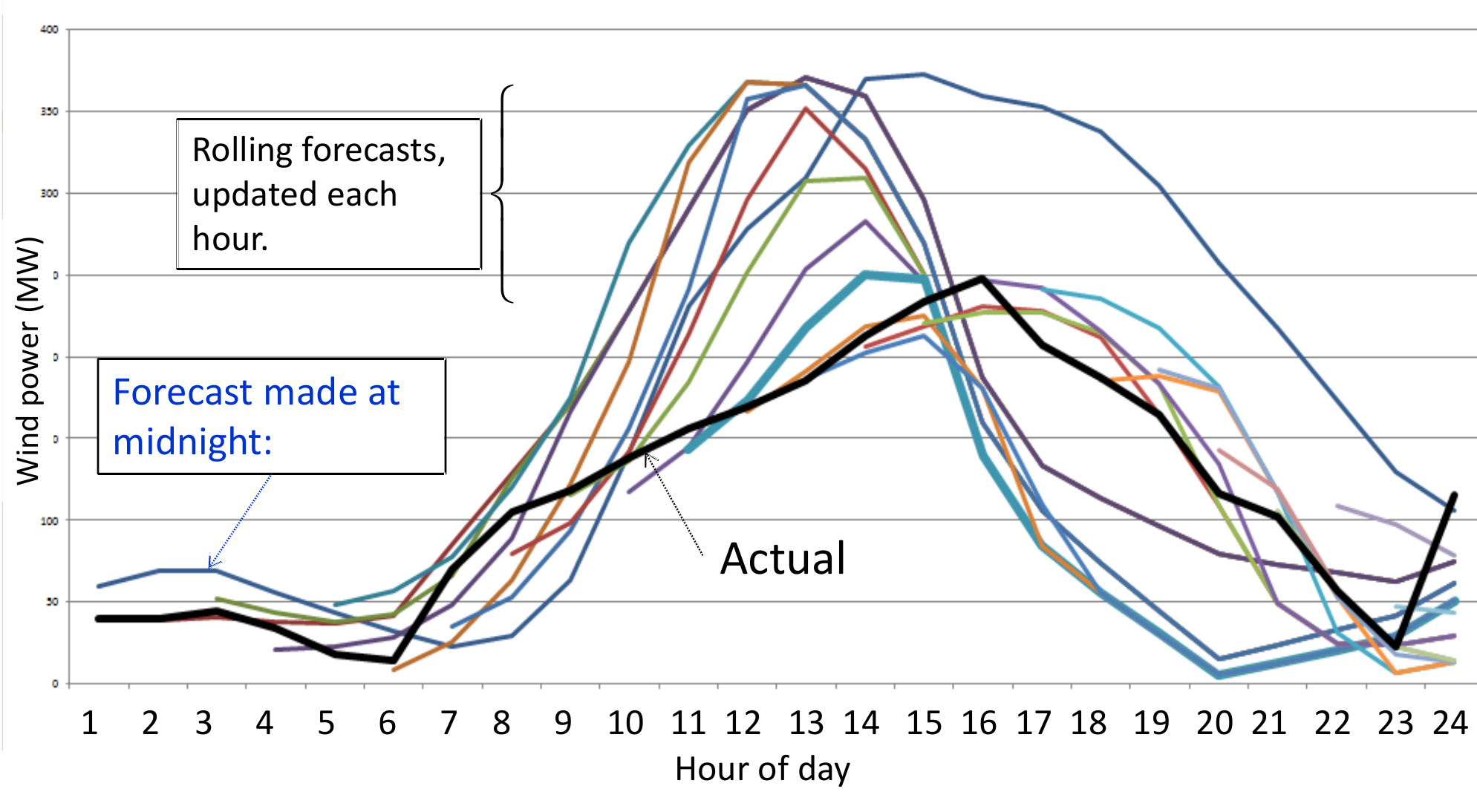
Each of these processes can be forecasted with varying degrees of accuracy. Forecasting wind power is the least accurate, and while wind can be stronger at night, highs and lows can occur at any time of the day or night. Loads are highly correlated with hour of day, largely because of human activity but also because of temperature. Note that hot afternoons can create peaks in the middle of a summer day from air conditioning, while it can actually reduce the heating load (which may be served by electrical heating) during the winter. Temperature also has a strong hour-of-day component due to the rising and setting of the sun, but there can be variations as weather fronts move through.

Our problem involves deciding how much to buy from the grid (or sell back to the grid) and how much to store at each point in time (these decisions might be made in 5-minute increments for some grid operators). We need to meet the demand for energy, but otherwise would like to maximize the revenue we make from selling energy minus the cost of buying the energy from the grid or wind farm.

Framing the problem

The answers to our three framing questions are:

• Metrics: We want to maximize the total expected profit which includes the revenue received from satisfying demand, minus the cost of purchasing energy from the grid.
• Decisions: We have six decisions: the flow of energy from the grid to storage, the flow of energy from the grid to the load, the flow of energy from the wind farm to storage, the flow of energy from the wind farm to the load, the flow of energy from the storage to the grid, and the flow of energy from the storage to the load.
• Uncertainties: We have the following dynamic information processes: the load (the demand for energy), the temperature (which influences the load), the energy from the wind farm, the price we receive from satisfying the load, and the cost of purchasing energy from the grid.

Basic model

State variables

We start by modeling the snapshot of the system at time $t$ which includes $R_t$, the amount of energy (in MWh) stored in the battery at time $t$; $L_t$, the load (demand) for energy at time $t$ (in MW); $\tau_t$, the temperature at time $t$; $w_t$, the energy from wind at time $t$ (in MW); $p^{load}_t$, the amount we are paid per MWh to satisfy the load to the building at time $t$; and $c^{grid}_t$, the cost of purchasing power from the grid (this is the price we are paid if we sell back to the grid).

Since the underlying problem is very time-dependent (due to daily cycles), we are going to need to use forecasts, both to model the dynamics of the problem as well as to make decisions which need to anticipate what might happen in the future. We assume that we are given a rolling set of forecasts as illustrated for wind in Figure 9.2. We model the forecasts for load ($L$), temperature ($\tau$), wind ($w$), market prices ($p$), and grid prices ($G$) using: $f^L_{tt’}$, the forecast of the load $L_t$ (in MW) at time $t’ > t$ given what we know at time $t$; $f^\tau_{tt’}$, the forecast of the temperature $\tau_t$ at time $t’ > t$ given what we know at time $t$; $f^w_{tt’}$, the forecast of the wind power $w_t$ (in MW) at time $t’ > t$ given what we know at time $t$; $f^p_{tt’}$, the forecast of market prices $p^{load}t$ (in $/MWh) at $t’ > t$ given what we know at time $t$; and $f^G{tt’}$, the forecast of grid prices $c^{grid}_t$ (in $/MWh) at $t’ > t$ given what we know at time $t$.

All forecasts are vectors over the horizon $t, t+1, \ldots, t+H$ where $H$ is a specified horizon (e.g. 24 hours). We let $f^X_t$ be the vector of forecasts for $X \in \Xcal = {L, T, W, P, G}$.

Our state variable is then

Here we have grouped the controllable resource $R_t$ (our physical state variable), the snapshot of load, temperature, wind power and price (which we might group as information variables $I_t$), and then the forecasts (which represent a form of belief $B_t$ about the future).

We quickly see that we have a relatively high-dimensional state variable. If we are planning in 5-minute increments, a rolling 24-hour forecast would have 288 elements. This hints at the challenge awaiting anyone who wants to estimate the value $V_t(S_t)$ of being in state $S_t$.

Decision variables

The decision variables for our system are now $x^{wr}_t$, the amount of power moved from the wind farm to the battery at time $t$; $x^{w\ell}_t$, the amount of power moved from the wind farm to the load (the building) at time $t$; $x^{gr}_t$, the amount of power moved from the grid to the battery at time $t$; $x^{rg}_t$, the amount of power moved from the battery to the grid at time $t$; $x^{g\ell}_t$, the amount of power moved from the grid to the load at time $t$; $x^{r\ell}_t$, the amount of power moved from the battery to the load at time $t$; and $x^{loss}_t$, uncovered load (known as “load shedding”).

These variables have to be determined subject to the constraints

Equation $\eqref{eq:energysystem1}$ limits the power to serve the load (the building) to the amount of the load (we cannot overload the building). The variable $x^{loss}$ captures the amount by which we have not covered the load. The constraint captures conversion losses for energy taken from the battery. Equation $\eqref{eq:energysystem2}$ says that we cannot move more power out of our battery storage than is in the battery, adjusted by conversion losses. Equation $\eqref{eq:energysystem3}$ then limits how much we can move into the battery to the amount of available capacity, again adjusted by the conversion losses. Equation $\eqref{eq:energysystem3a}$ limits how much we can move from the storage back to the grid. Equation $\eqref{eq:energysystem4}$ limits the amount from the wind farm to what the wind farm is generating at that point in time. Equations $\eqref{eq:energysystem5}$–$\eqref{eq:energysystem6}$ limit the flows into and out of the battery to charge and discharge rates. Equation $\eqref{eq:energysystem7}$ imposes nonnegativity on each variable.

Exogenous information

Our first source of exogenous information is the difference between the actual and forecasted value for any process “$X$” where

Let $X_t$ be the process and $\varepsilon^X_{t+1}$ be the difference between the actual and forecasted values. We then let

We might model $\varepsilon^X_{t+1}$ using samples drawn from historical data, or by assuming it follows some assumed distribution.

The second source of exogenous information is the change in forecasts as we step forward in time. We again let $f^X_t$ be a vector of forecasts for each information process $X$, where $f^X_{tt}$ is the actual value at time $t$. Let $\fhat^X_{t+1,t’}$ be the change in the forecast for time $t’$ between $t$ and $t+1$, so that

The exogenous changes $\fhat^X_{t+1,t’}$ are correlated across the time periods $t’$. If this were not the case, then the forecasts when plotted over the horizon $t’=t, \ldots, t+H$ would no longer exhibit the smoothness that we see in the wind forecasts in Figure 9.2. We return to the issue of modeling the uncertainty in forecasts below.

This means we can write our exogenous information as

for $X$ equal to the different variables (load, temperature, wind, market prices and grid prices).

Transition function

The evolution of the resource state variable is given by

Each of the variables $L_t$, $\tau_t$, $w_t$, $p^{load}_t$, and $c^{grid}_t$ evolve using the forecasts. For example, we would write the evolution of the load $L_t$ using

We could create similar equations for $\tau_t$, $w_t$, $p^{load}_t$, and $c^{grid}_t$.

We write the evolution of the forecasts using

for $X=L, \tau, w, p^{load}$ and $c^{grid}$. Equation $\eqref{eq:energytransitionII3}$ is known in the literature as the “martingale model of forecast evolution.” The term “martingale” refers to our assumption that $f^X_{tt’}$ is an unbiased estimate of $f^X_{t+1,t’}$ since we assume that the random deviations $\fhat^X_{t+1,t’}$ are, on average, zero.

Equations $\eqref{eq:energytransitionII1}$, $\eqref{eq:energytransitionII2}$ and $\eqref{eq:energytransitionII3}$ (for all forecasts $X$) make up the transition function

Objective function

Our profit function at time $t$ is given by

where the market price $p^{load}_t$ and grid price $c^{grid}_t$ are contained in the state variable $S_t$. Our objective function is still the canonical problem given by

As before, $S_{t+1} = S^M(S_t,X^\pi(S_t),W_{t+1})$ which is given by equations $\eqref{eq:energytransitionII1}$, $\eqref{eq:energytransitionII2}$ and $\eqref{eq:energytransitionII3}$.

Modeling uncertainty

We describe below two styles for modeling uncertainty over time. We first describe a method for modeling the correlations in errors in the forecasts over time using a technique sometimes called Gaussian process regression. This method ensures that as we move forward in time, a vector of forecasts evolves in a natural way.

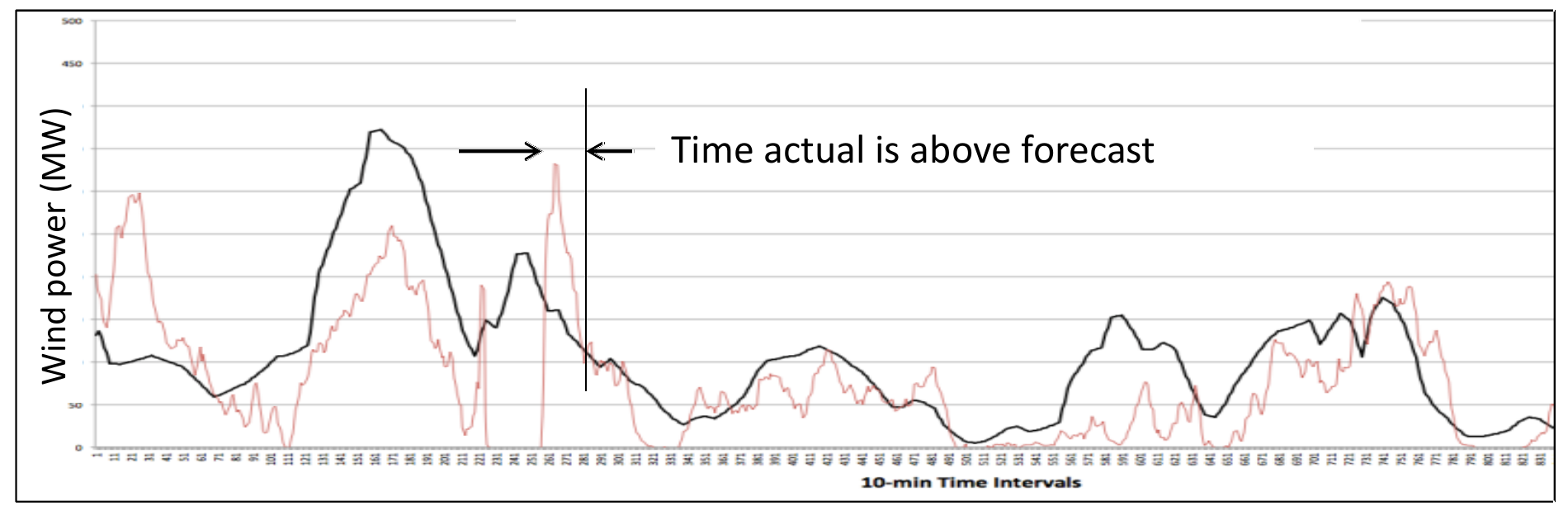
Then we describe a hidden-state Markov model that we have found provides exceptionally realistic sample paths for stochastic processes. This model closely replicates error distributions, but also does a very nice job capturing crossing times, which is the time that the actual process (e.g. wind speed) stays above or below a benchmark such as a forecast. If we can properly capture the time that a forecast is above or below the actual, then it means we are capturing correlations over time.

This section will illustrate several powerful methods for stochastic modeling that should be in any toolbox for modeling uncertainty. Stochastic modeling can be technically sophisticated, and this section reflects this. The reader is warned that this section is much more involved than our other sections on modeling uncertainty.

Gaussian process regression for forecast errors

Gaussian process regression (GPR for short) is a simple method for generating correlated sequences of normally distributed random variables. GPR is particularly useful when trying to estimate a continuous surface, where if one point in the surface is higher than expected, then it means that nearby points will also be higher than expected.

Let $X_{t’}$ be the actual outcome of any of our exogenous processes (prices, loads, temperature, wind energy) at time $t’$, and let $f^X_{tt’}$ be the forecast of $X_{t’}$ made at time $t < t’$. It is common to assume some error $\varepsilon_{t’-t}$ that describes the difference between $X_{t’}$ and the forecast $f^X_{tt’}$. We would then assume some model for $\varepsilon^X_{t’-t}$ such as

We are going to take a somewhat different approach by assuming that the distribution in the change in a forecast $\fhat^X_{t+1,t’}$ is described by

We then assume that the changes in the forecasts $\fhat^X_{t+1,t’}$ are correlated across times $t’$ with a covariance function

The covariance function $Cov(\fhat^X_{t+1,t’},\fhat^X_{t+1,t’’})$ in equation $\eqref{eq:forecastcovariancefunction}$ captures the property that the covariance across time exhibits correlations that decrease with the difference between the two points in time. This simple model introduces the tunable parameter $\beta$ that has to be estimated from data, or possibly by judgment. For example, it might be possible to plot the covariance values for different values of $\beta$ and choose one that seems reasonable.

We can use this covariance function to create a covariance matrix $\Sigma^X$ with element $\Sigma^X_{t’t’’} = \sigma^2_X e^{-\beta\vert t’‘-t’\vert }$. There is a simple way of creating a correlated sample of changes in forecasts using a method called Cholesky decomposition. It begins by creating what we might call the “square root” of the covariance matrix $\Sigma^X$ which we store in a lower triangular matrix $L$. In python, using the NumPy package, we would use the python command

L = scipy.linalg.cholesky(Sigma_X, lower=True)

We note that $\Sigma^X = L^T L$, which is why we think of $L$ as the square root of $\Sigma^X$.

Next generate a sequence of independent random variables $Z_{\tau}$ for $\tau = 1, \ldots, H$ that are normally distributed with mean 0 and variance 1. Now let $Z=(Z_{t+1}, Z_{t+2}, \ldots, Z_{t+H})^T$ be a column vector made up of these independently distributed standard normal random variables. We can create a correlated sample of changes in the forecasts using

This formula gives us a sampled set of changes in forecasts $\fhat^X_{t+1,t+1}, \ldots, \fhat^X_{t+1,t+H}$ that are correlated according to our exponential decay function in equation $\eqref{eq:forecastcovariancefunction}$. The result will be an evolving set of forecasts where the variance in the errors in the forecasts grows linearly over time according to

The evolving forecasts $f^X_{t,t’}, f^X_{t+1,t’}, \ldots$ will exhibit the behavior that we saw in our evolving wind forecasts in Figure 9.2.

Hidden-state Markov model

A challenge when developing stochastic models in energy is capturing a property known as a crossing time. This is the time that an actual process (e.g. price or wind speed) is above or below some benchmark such as a forecast. Figure 9.3 illustrates an up-crossing time for a wind process.

Replicating crossing times using standard time series modeling proved unsuccessful. What did work was the development of a Markov model with a hidden state variable $S^C_t$ which is calibrated to capture the dynamics of the process moving above or below the benchmark. The process uses the following steps:

Step 1 – Comparing the actual process to the benchmark, find the times at which the actual process moves above or below the benchmark, and output a dataset that captures whether the process was above (A) or below (B) and for how long. Aggregate these periods into three buckets (S/M/L) for short/medium/long, and label each segment with A or B and S/M/L, creating six states. These are called “hidden states” because, while we will know at time $t$ if the actual process is above or below the benchmark, we will not know if the length is short, medium or long until after the process crosses the benchmark.

Step 2 – Using the historical sequence of $S^C_t$, compute a one-step transition matrix $P^C[S^C_{t+1}\vert S^C_t]$, the probability that the crossing process takes on value $S^C_{t+1}$ given that it is currently in state $S^C_t$.

Step 3 – Aggregate the actual process (e.g. wind speed) into, say, five buckets based on the empirical cumulative distribution. Let $W^g_t$ be the aggregated wind speed (a number from 1 to 5).

Step 4 – From history, compute the conditional distribution of wind speed given $W^g_t$ and $S^C_t$, $F^W[W_{t+1}\vert W^g_t, S^C_t]$, the empirical cumulative distribution of the wind speed $W_{t+1}$ given $W^g_t$ and $S^C_t$.

Using the one-step transition matrix $P^C[S^C_{t+1}\vert S^C_t]$ and the conditional cumulative distribution $F^W[W_{t+1}\vert W^g_t, S^C_t]$, we can now simulate our stochastic process by first simulating the hidden state variable $S^C_{t+1}$ given $S^C_t$ (note that there are only 30 of these). Then, from a wind speed $W_t$, we can find the aggregated wind speed $W^g_t$, and then sample the actual wind speed $W_{t+1}$ from the conditional cumulative distribution $F^W[W_{t+1}\vert W^g_t, S^C_t]$.

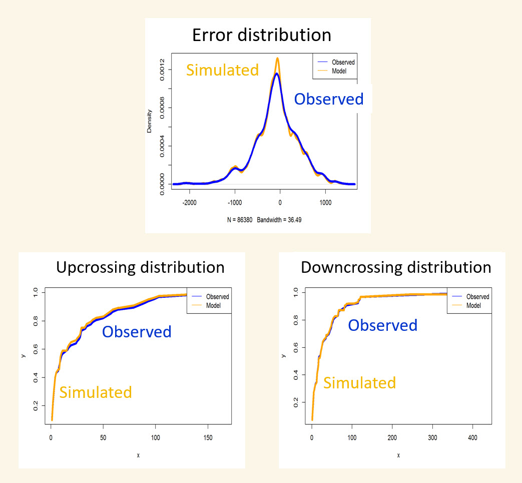
This logic has been found to accurately reproduce both the error distribution (actual vs. benchmark), as well as both up-crossing and down-crossing distributions across a range of datasets modeling wind as well as grid prices. Figure 9.4 illustrates these distributions on a particular dataset.

Designing policies

The biggest complication of this problem is that the forecasts are part of the state variable, which allows us to explicitly model the rolling evolution of the forecast. The difficulty is that this makes the state variable high-dimensional.

The most common approaches for handling forecasts use a lookahead model that approximates the future by fixing the forecast. The two most popular strategies are:

• Deterministic lookahead with the forecast captured in the formulation of the lookahead.
• Stochastic lookahead with latent variables – We can use the forecast to develop a stochastic lookahead model which we then solve using classical dynamic programming. In the lookahead model, we fix the forecasts into the model, rather than modeling their evolution over time. When we ignore a variable in a model (including a lookahead model), it is called a latent variable.

Both of these methods use the forecast as a latent variable in that they do not model the evolution of the forecast within the lookahead model. The difficulty with the stochastic lookahead model is that it is harder to solve. If we are optimizing our energy storage problem in short-time increments (this might be 5-minutes, or even less), then this can create problems for techniques such as exact or even approximate dynamic programming.

For this reason, the most popular strategy for handling time-dependent problems with a forecast is to solve a deterministic lookahead model, just as we did for our dynamic shortest path problem. We describe such a model below, and then introduce a parameterized version that allows the deterministic model to better handle uncertainty.

We pause to note that planning using rolling forecasts is quite common in operations management. Oddly, textbooks almost uniformly ignore the proper modeling of rolling forecasts. Virtually every book on inventory planning, for example, equates the state variable with the inventory. Only a small handful recognize that if forecasts are being updated each time period, then we have to represent the information needed to update the forecasts in the state variable. If we ignore this information, then we are effectively creating a lookahead model where the forecast is being held constant.

Deterministic lookahead

We are going to use the same notational style we first introduced in Chapter 6, where we distinguish our base model, which is the problem we are trying to solve, from the lookahead model which we solve as a form of policy for solving the base model.

Recall that the canonical formulation of our base model is

where $S_{t+1} = S^M(S_t,X^\pi(S_t),W_{t+1})$, and where we have an exogenous information process $(S_0, W_1, W_2, \ldots, W_T)$. Note that the variables $W_t$ may depend on the state $S_t$ and/or decision $x_t$; if this is the case, then the variable $W_{t+1}$ has to be generated on the fly after we know $S_t$ and $x_t$.

We are going to create a policy by formulating a deterministic lookahead model, where all the variables are labeled with tildes, and indexed both by the time $t$ at which we are making our decision, and time $t’$ which is the time variable within the lookahead model. So we would define $\xtilde_{tt’}$, the decision at time $t’$ in the lookahead model being generated at time $t$; $\ctilde_{tt’}$, the cost coefficient for $\xtilde_{tt’}$; and $\Rtilde_{tt’}$, the energy in the battery at time $t’$ in the lookahead model generated at time $t$.

Note that $x_t = \xtilde_{tt}$, $c_t = \ctilde_{tt}$ and so on.

We create our deterministic lookahead policy $X^{DLA}_t(S_t)$ as the following linear program:

where

This problem has to be solved subject to the constraints $\eqref{eq:energysystem1}$–$\eqref{eq:energysystem7}$ for $x_t$, and the following constraints for $\xtilde_{tt’}$ for all $t’ = t+1, \ldots, t+H$:

These equations mirror the ones in the base constraints $\eqref{eq:energysystem1}$–$\eqref{eq:energysystem7}$, with the only change that we use the lookahead variables such as $\xtilde_{tt’}$, $\Rtilde_{tt’}$, and forecasts such as $f^W_{tt’}$ instead of the actual wind $W_t$.

The model described by equations $\eqref{eq:energydetlookahead0}$–$\eqref{eq:energydetlookahead8}$ is a relatively simple linear program, for which packages are now available in languages such as Matlab or python.

Lookahead policies such as $X^{DLA}_t(S_t)$ are widely used in dynamic, time-varying problems such as this. They have to be solved on a rolling basis as we first illustrated for our deterministic shortest path problem. For this reason, these are sometimes called “rolling horizon procedures” or “receding horizon procedures.” There is an entire field known as “model predictive control” which is based on these lookahead policies.

For applications such as this energy storage problem, the use of a deterministic lookahead model raises the concern that we are not accounting for uncertainties. For example, we might want to store extra energy in the battery to protect ourselves from a sudden drop in wind or a surge in prices on the grid. In the next section, we are going to describe how to use a deterministic lookahead model to handle uncertainty.

Parameterized lookahead

There is a very simple way to address the problem that our deterministic lookahead does not handle uncertainty. What we need to do is to think about how we might modify the model (or the solution) because of uncertainty. For example, we might wish to pay for extra storage in the future to handle unexpected variations. Of course, we cannot force the model to keep energy in storage right now when we might need it. We might also want to discount forecasts that might not be very accurate.

We can introduce these changes by replacing the constraints $\eqref{eq:energydetlookahead1}$–$\eqref{eq:energydetlookahead8}$ with the following

Note that we have introduced parameters to modify the right hand side of constraints $\eqref{eq:energydetlookaheadmod2}$ and $\eqref{eq:energydetlookaheadmod5}$ where we have introduced coefficients $\theta^L_{t’-t}$ and $\theta^W_{t’-t}$ to modify the forecasts of load and wind, where the coefficients are indexed by how many time periods we are forecasting into the future. Then, we modified the constraint $\eqref{eq:energydetlookaheadmod3}$ with the idea that we may want to restrict our ability to use all the energy in storage in order to maintain a reserve.

Let $X^{DLA-P}(S_t\vert \theta)$ represent the lookahead policy that is solved subject to the parameterized constraints $\eqref{eq:energydetlookaheadmod1}$–$\eqref{eq:energydetlookaheadmod8}$. Once we have decided how to introduce these parameterizations (this is the art behind any parametric model), there is the problem of finding the best value for $\theta$. This is the problem of parameter search that we addressed in Chapter 7.

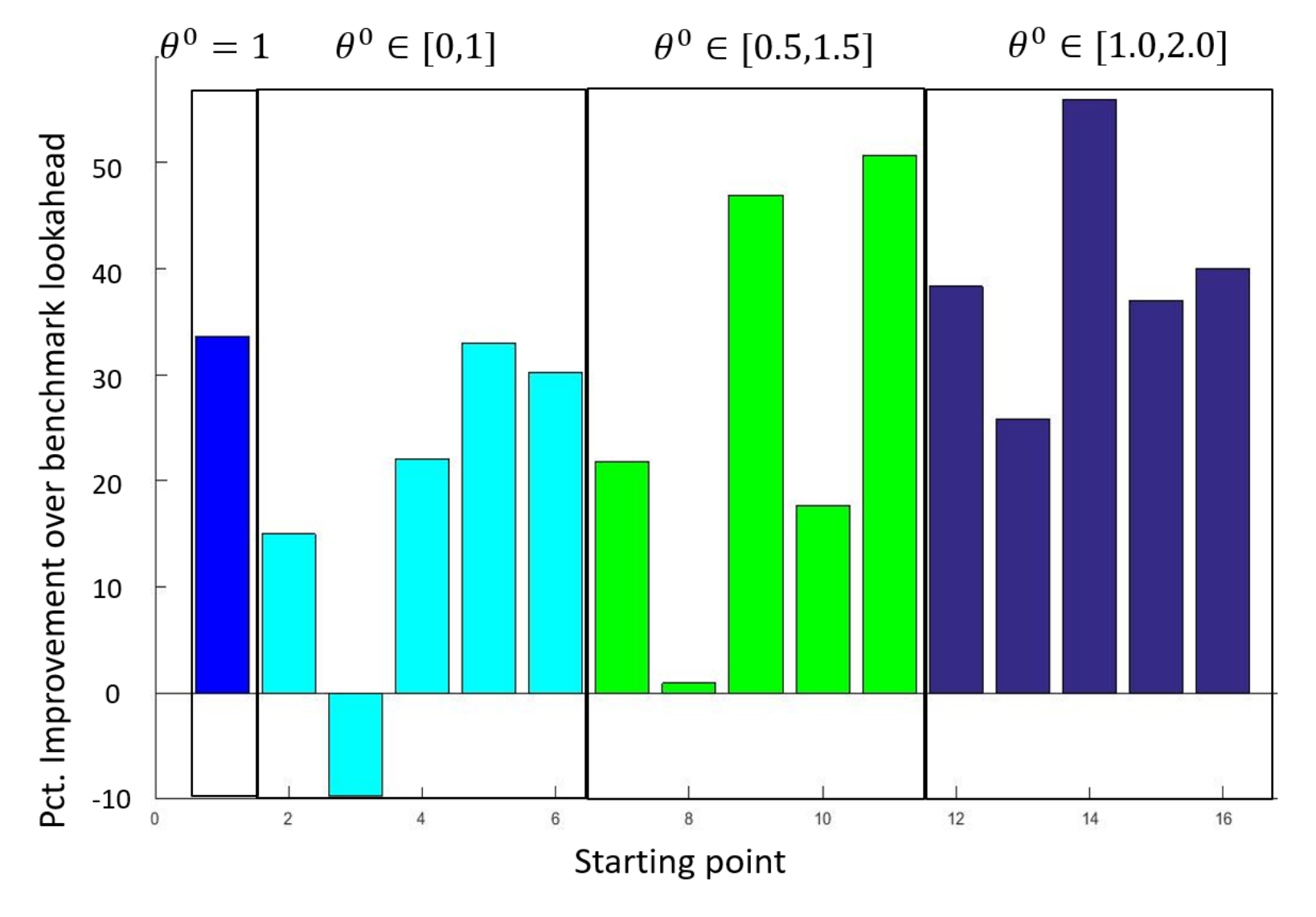
We computed the relative improvement from using an optimized, parameterized deterministic lookahead, where we search for the best values of the vector $\theta=(\theta^L, \theta^W)$, versus a basic policy that sets these parameters equal to 1.0. In our experiments, we set $\theta^L_{t’-t} = 1$, and just optimized the coefficient of the wind forecast, $\theta^W_{t’-t}$.

The results are shown in Figure 9.5, which show that we improve performance on average by about 30 percent. What is important is that this improvement does not come with any additional complexity when making decisions in the field. The only step, which we have not described here, is that we have to tune the parameter vector $\theta$. The process of optimizing $\theta$ is, unfortunately, not easy.

What did we learn?

• In this chapter we introduce a much more complex energy storage problem with rolling forecasts.
• We introduce the “martingale model of forecast evolution” which assumes that forecasts of the future evolve over time, where the expected change in a forecast is zero (but the actual change is positive or negative).
• We then describe a hidden semi-Markov model that helps us replicate “crossing times” which capture the time that a forecast is above or below actual.
• We introduce a deterministic lookahead policy, and then a parameterized deterministic lookahead, where we introduce coefficients for each forecast (another example of a hybrid DLA/CFA).
• We show that the tuned DLA/CFA policy outperforms the pure (untuned) deterministic lookahead by around 30 percent.

Exercises

Review questions

1. What is meant by the "martingale model of forecast evolution"?
2. The entire forecast at time $t$ for each quantity such as the load $L_t$, $f^L_{tt'}$ for $t'=t, \ldots, t+H$, are in the state variable. Why? [Hint: look at the transition equations for forecasts and the variables they are forecasting.]
3. What is the difference between the variables $x_t$, $t=0, \ldots, T$, and the variables $\xtilde_{tt'}$ for $t' = t, \ldots, t+H$?
4. What is a "crossing time"?
5. What is a "Cholesky decomposition" and what is it used for?
6. What state is hidden in the hidden-state Markov model of wind energy? Explain why it is hidden.
7. What class of policy is the parameterized lookahead policy above? What objective function is used for finding the best set of tuning parameters?

Problem solving questions

1. Try designing a parameterized policy for making decisions under the conditions of the problem in this chapter. You may use anything in the form of rules or parameterized functions. The only limitation is that you are not allowed to optimize over anything (which is to say, you cannot use an $\argmax_x$ within your policy).
2. Our parameterized lookahead was limited to introducing coefficients in front of forecasts. You may also introduce additive adjustments, such as keeping the energy storage device from getting too close to its capacity (this would allow you to store a burst of wind that exceeds the forecast) or from getting too close to zero (in case you have a dip in the wind). Suggest an alternative parameterization and make an argument why your structure might add value.