Chapter 8: Energy storage I

Chapter overview

This chapter considers what initially looks like a fairly simple inventory problem that arises when storing energy that we can buy from or sell to the grid, which features highly stochastic prices. In contrast with the first six chapters, we use a much richer set of models for describing these stochastic prices which starts to hint at the complexity that we can encounter when modeling uncertainty. We provide a tour through different models for price processes, including classical time series models, jump diffusion models (for capturing spikes), quantile distributions, and finally a hybrid that combines quantile distributions with standard normal distributions, opening the door to using methods that depend on normality.

We then describe a series of policies, starting with a basic “buy low, sell high” policy (a form of policy function approximation) before transitioning to several methods based on approximating Bellman’s equation, which we first saw in Chapter 5. We start with a vanilla description of Bellman’s equation (which is computationally infeasible for almost all problems), and then provide a tour through variations known as backward approximate dynamic programming (ADP), forward ADP, and a hybrid strategy using forward ADP combined with parameter tuning.

Narrative

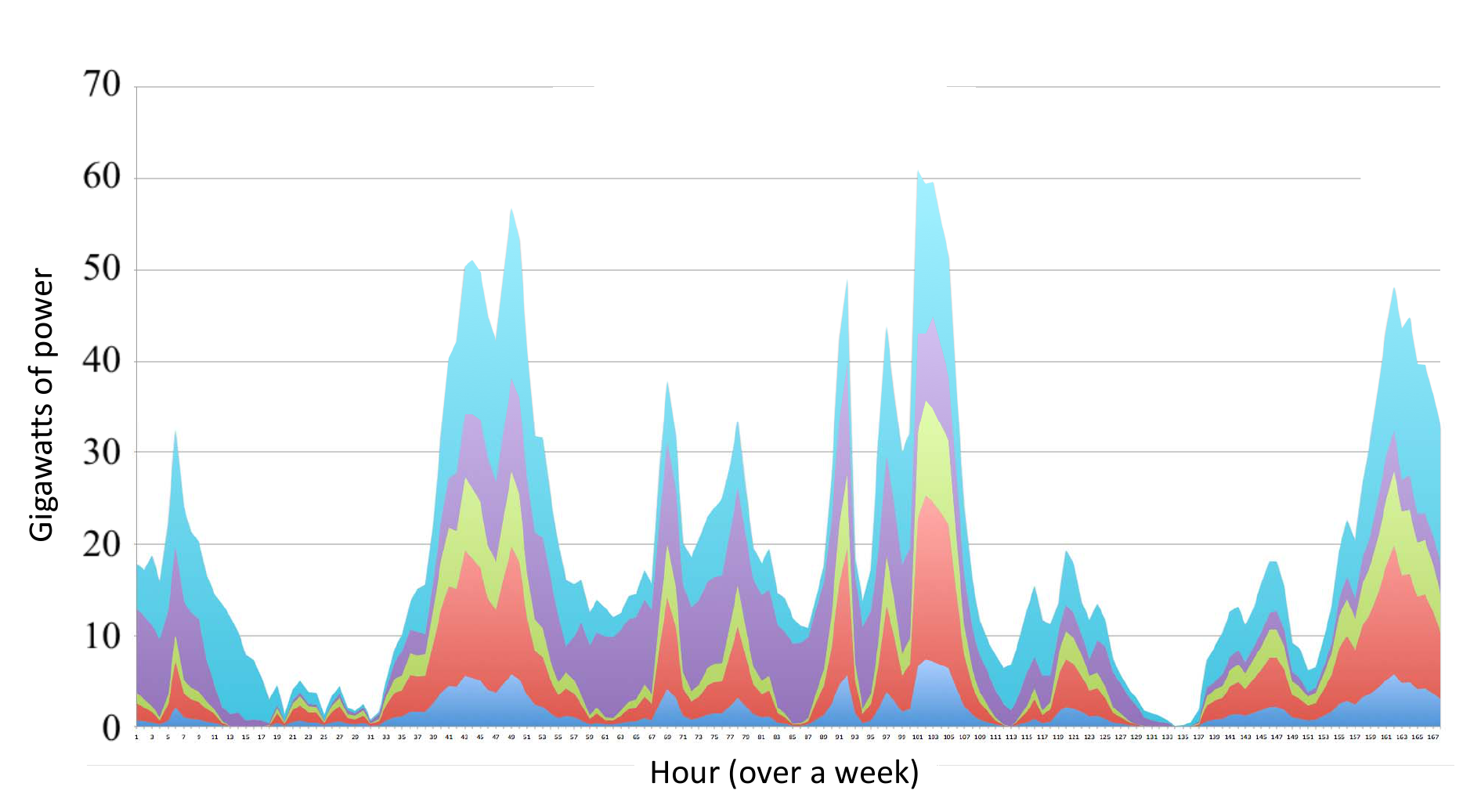
New Jersey is looking to develop 3,500 megawatts (MW) of off-shore wind generating power. A challenge is that wind (and especially offshore wind) can be highly variable. The effect of this variability on the power grid is magnified by the property that wind power (over intermediate ranges) increases with the cube of wind speed. This variability is depicted in Figure 8.1.

Energy from wind power has become popular in regions where wind is high, such as the midwestern United States, coastal regions off of Europe, the northeast of Brazil, and northern regions of China (to name just a few). Sometimes communities (and companies) have invested in renewables (wind or solar) to help reduce their carbon footprint and minimize their dependence on the grid.

It is quite rare, however, that these projects allow a community to eliminate the grid from their portfolio. Common practice is to let the renewable source (wind or solar) sell directly to the grid, while a company may purchase from the grid. This can be useful as a hedge since the company will make a lot of money during price spikes (prices may jump from $20 per megawatt-hour (mwh) to $300 per mwh or more) that offsets the cost of purchasing power during those periods.

The major difficulty with renewables is handling the variability. While one solution is to simply pump any energy from a renewable source into the grid and use the capacity of the grid to handle this variability, there has been considerable interest in using storage (in particular, battery storage) to smooth out the peaks and valleys. In addition to smoothing the variability in the renewable source, there has also been interest in using batteries to take advantage of price spikes, buying power when it is cheap (prices can even go negative) and selling it back when they are high. Exploiting the variability in power prices on the grid to buy when prices are low and sell when they are high is known as battery arbitrage.

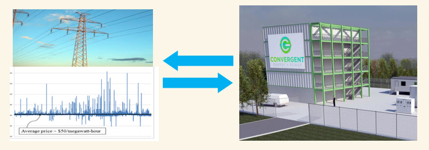
We are going to use the configuration shown in Figure 8.2 to illustrate a number of modeling and algorithmic issues in energy storage. This problem will provide insights into virtually any inventory/storage problem, including:

• Holding cash in mutual funds – A bank has to determine how much of its investment capital to hold in cash to meet requests for redemptions, versus investing the money in loans, stocks and bonds.
• Retailers (including both online as well as bricks-and-mortar stores) have to manage inventories of hundreds of thousands of products.
• Auto dealers have to decide how many cars to hold to meet customer demand.
• Consulting firms have to decide how many employees to keep on staff to meet the variable demand of different consulting projects.

Energy storage is a particularly rich form of inventory problem. While we are not going to consider all possible variations (which are endless), our problem will exhibit the following characteristics:

• Electricity prices on the grid can be highly volatile. In the early 2000s, typical energy prices ran around $20-$25 per mwh, but often spiked to over $300, and could exceed $1000, typically during extreme weather events.
• Energy from wind can be forecasted, although not very well. Rolling forecasts are available to update these estimates.
• Solar energy exhibits three types of variability: the highly predictable process of the diurnal cycle of the sun rising and setting, the presence of very sunny or very cloudy days (these can typically be predicted a day or more in advance), and the variability of spot clouds that are difficult to predict even an hour into the future, but which can create severe power surges on the grid.
• The demand for energy is variable, but relatively predictable, since it primarily depends on temperature (and, to a lesser extent, humidity).
• Energy may be bought from or sold to the grid at current grid prices. Similarly energy from the renewables source may be used to satisfy the current load (demand for power), stored, or sold back to the grid (depending on the configuration).
• There is a roughly 5 to 10 percent loss for the conversion of power from AC (as it arrives over the grid) to DC (required to store power in the battery).

Framing the problem

The answers to our three framing questions are:

• Metrics: We wish to minimize the expected price we pay for electricity purchased from the grid.
• Decisions: The amount of energy we purchase each time period from the grid, or sell back to the grid.
• Uncertainties: The price of electricity at each time period.

Basic model

We will use a sequence of variations of this problem to illustrate different modeling issues, beginning with a basic system of using a battery to buy from and sell to the grid to take advantage of price volatility. For this application, we will step forward in 5-minute time increments, since this is the frequency with which prices are updated on the grid (this time increment varies depending on the grid operator).

State variables

For our basic model, we only need to keep track of two variables: $R_t$, the amount of energy (measured in megawatt-hours, or mwh) stored in the battery at time $t$; and $p_t$, the price of energy on the grid. Our state variable is then

The state variable quickly becomes more complex as we add different elements to the model. For example, the state variable to represent prices depends on how we model the price process, as described in the transition function (see below).

Decision variables

Our only decision is whether to buy from or sell to the grid: $x_t$, the amount of power bought from ($x_t > 0$) or sold to ($x_t < 0$) the grid.

When we transfer energy into or out of the battery, we are going to assume that we only get a fraction $\eta$ in the transfer, implying a loss of $1-\eta$. For simplicity we are going to assume that this loss is the same regardless of whether we are charging or discharging the battery.

The decision is limited by the capacity of the battery, which means we have to observe the constraints

where the first constraint applies when we are buying from the grid ($x_t > 0$) while the second constraint applies when we are selling to the grid ($x_t < 0$).

As always, we assume that decisions are made with a policy $X^\pi(S_t)$, to be determined below.

Exogenous information

In our basic model, the only exogenous information is the change in prices. We may assume that the price in each time period is revealed, without any model to predict the price based on past prices. In this case, our exogenous information $W_t$ would be

Alternatively, we can assume that we observe the change in price $\phat_t = p_t - p_{t-1}$, in which case we would write

Transition function

The evolution of the state variables is given by

This style of modeling the price process by “observing” the change in price helps us when writing the transition function. In practice, we would typically be observing $p_{t+1}$ directly (rather than the change), in which case there is no need for an explicit transition equation. These two equations make up our transition function $S_{t+1} = S^M(S_t,x_t,W_{t+1})$.

Later, we are going to find it useful to model the post-decision state $S^x_t$, which is the state just after we make a decision $x_t$, but before any new information arrives. The post-decision resource state is

Because the storage variable evolves deterministically, the transition to the next pre-decision state is just

The price $p_t$, on the other hand, is not affected by the decision, so the post-decision price would just be

This means the post-decision state is

Objective function

In any period, the amount of money we make or lose is given by

Our objective function is then the canonical problem given by

where $S_{t+1} = S^M(S_t,X^\pi(S_t),W_{t+1})$ is given by equations $\eqref{eq:energytransition1}$ and $\eqref{eq:energytransition2}$. We then also need to specify the initial state $S_0$ (that is, $R_0$ and $p_0$) and have a method for generating $W_1, W_2, \ldots$, which we describe next.

Modeling uncertainty

In our asset selling problem in Chapter 2, we assumed that we could model prices according to

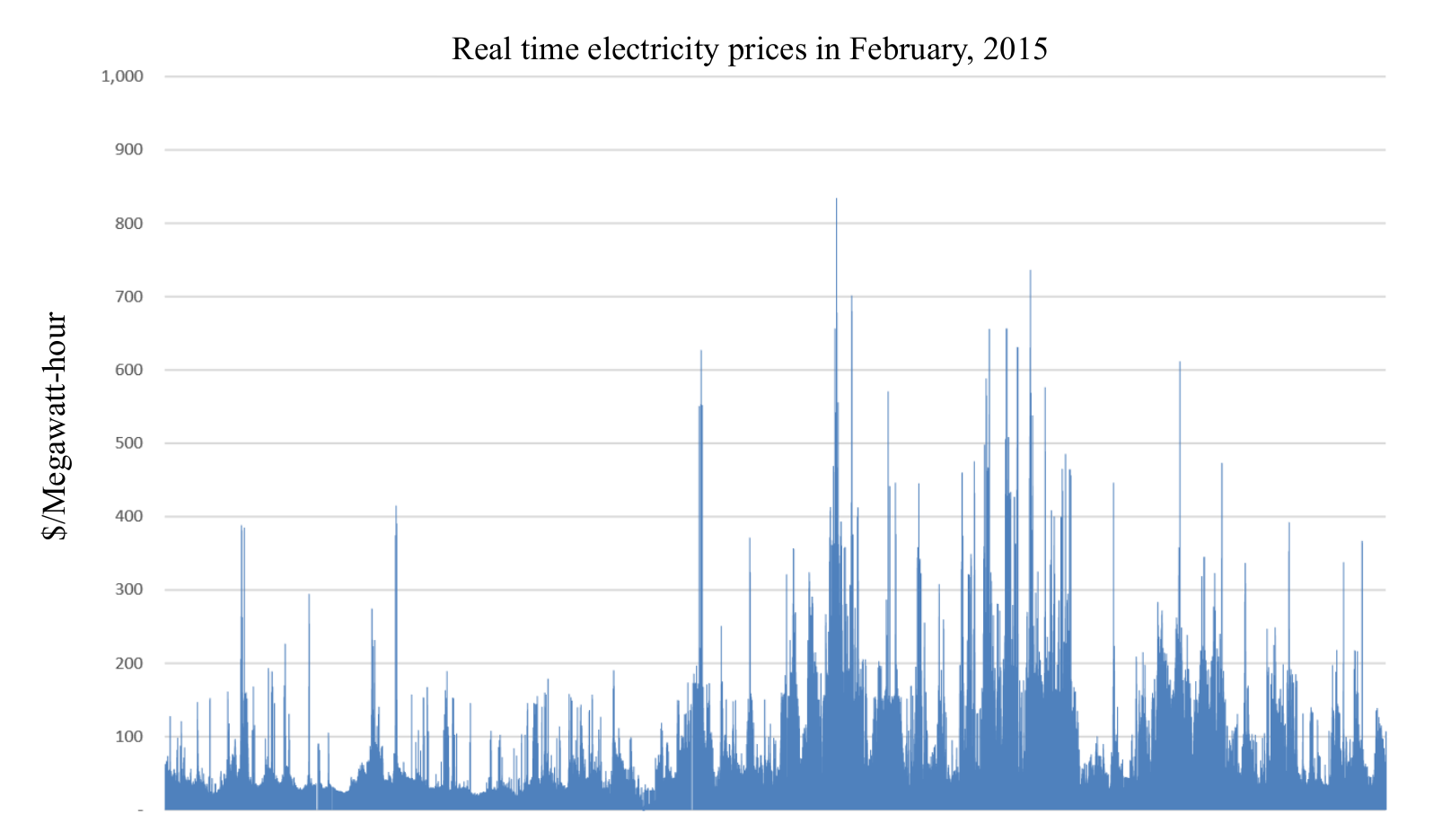
where we then assumed that $\varepsilon_{t+1}$ was normally distributed with mean 0 and some known variance. Figure 8.3 shows grid prices, known as “locational marginal prices” (or LMPs in the terminology of the power community) over a year, which illustrates the tremendous volatility that prices on the grid exhibit. This volatility arises because there are surges in load (or losses in power) that can create short term shortages. Since demand is inelastic (the grid is supposed to meet 100 percent of the load), prices can jump by a factor of 20 to 50 for short periods (prices are updated in 5-minute increments).

There are several methods for modeling electricity prices. Below we are going to describe four that have been used for this problem.

Time series models

The time series literature is quite rich, so we are just going to illustrate a basic model which represents the price $p_{t+1}$ as a function of the recent history of prices. For illustration, we are going to use the last three time periods, which means that we would write our model as

where

is our vector of prices. We assume that the noise $\varepsilon \sim N(0,\sigma^2\epsilon)$ for a given $\sigma^2\epsilon$.

The vector of coefficients $\thetabar_t = (\thetabar_{t0},\thetabar_{t1},\thetabar_{t2})^T$ can be estimated recursively. Assume that we start with an initial estimate $\thetabar_0$ of the vector of coefficients. We are also going to need a three-by-three matrix $M_0$ that for now we can assume is a scaled identity matrix (we provide a better idea below).

The basic updating equation for $\thetabar_t$ is given by

The error $\hat{\varepsilon}_t$ is computed using

The three-by-three matrix $H_t$ is computed using

where the matrix $M_t$ is computed recursively using

The variable $\gamma_t$ is a scalar computed using

These equations need initial estimates for $\thetabar_0$ and $M_0$. One way to do this is to collect some initial data and then solve a static estimation problem. Assume you observe $K$ prices. Let $Y_0$ be a $K$-element column vector of the observed prices $p_3, p_4, \ldots, p_{K+3-1}$ (we have to start with the third price because of our need for the trailing three prices in our model).

Then let $X_0$ be a matrix with $K$ rows, where each row consists of $p_k, p_{k-1}, p_{k-2}$. Our best estimate of $\thetabar$ is given by the normal equations

Finally let $M_0 = [(X_0)^T X_0]^{-1}$, which shows that the matrix $M_t$ is the time $t$ estimate of $[(X_t)^T X_t]^{-1}$.

There are entire families of time series models that capture the relationship of variables over time. If we were to just apply these methods directly to price data, the results would be quite poor. First, the prices are not normally distributed. Second, while prices may go negative, this is fairly rare. However, a direct application of this model would be very likely to produce negative prices if the variance $\sigma^2_\epsilon$ was calibrated to the high-noise of this type of data. Finally, the behavior of the jumps in prices over time would not be realistic.

Jump diffusion

A major criticism of the linear model above is that it does a poor job of capturing the large spikes that are familiar in the study of electricity prices. A simple idea for overcoming this limitation is to use what is known as a jump diffusion model, where we add another noise term to equation $\eqref{eq:energytimeseriesmodel}$ giving us

Here, the indicator variable $\mathbb{I}t = 1$ with some probability $p^{jump}$, and the noise $\varepsilon^J{t+1}$ is normally distributed with mean $\mu^{jump}$ (which is typically much larger than zero) and variance $(\sigma^{jump})^2$ which is quite large.

We have to estimate the jump probability $p^{jump}$, and the mean and variance $(\mu^{jump}, (\sigma^{jump})^2)$. This is done by starting with a basic model where $p^{jump} = 0$. We use this basic model to estimate $\sigma^2\epsilon$. We then choose some tolerance such as three standard deviations (that is, $3 \sigma\epsilon$), and any observations outside of this range are due to a different source of noise. Let $p^{jump}$ be the fraction of time periods where these observations occur. Then, compute the mean and standard deviation of these observations to get $(\mu^{jump}, (\sigma^{jump})^2)$.

We do not stop here. After taking these extreme variations from the data, we should re-fit our linear model without these observations. Standard practice is to repeat this process several times until these estimates stop changing.

Jump diffusion models do a better job of replicating the tails, but it still depends on the tail behavior of the normal distribution. A better fit can be obtained by recognizing that the variance of the noise depends on the temperature, and particularly on extreme temperatures. We might group temperatures into three ranges: below freezing, above 90 degrees F, and in-between these two values. Introducing temperature dependence, while adding another variable to the set of state variables, does introduce an additional degree of complexity (the effect of this depends on the class of policy).

Quantile distributions

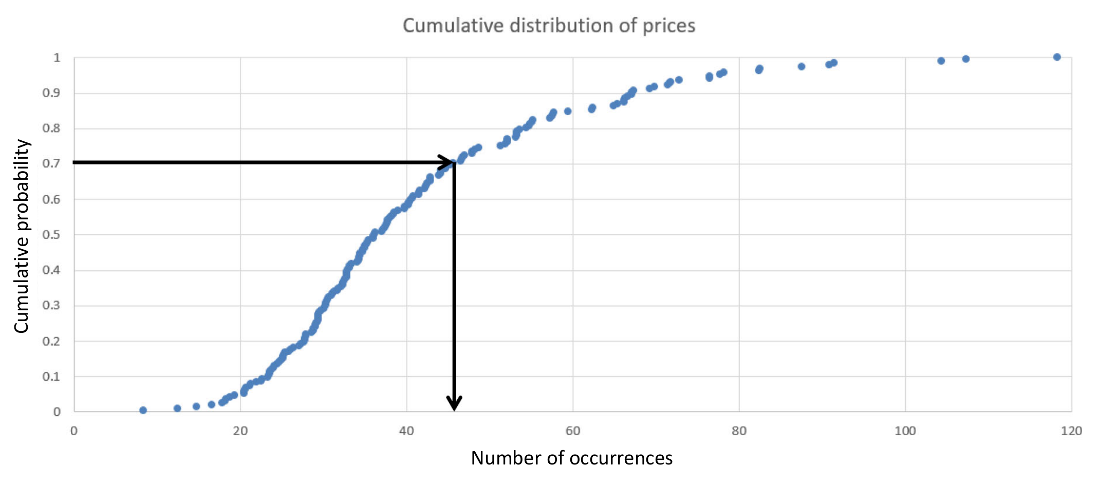
While it may be possible to fit other parametric distributions, a powerful strategy is to numerically compute the cumulative distribution from the data, creating what is often called a quantile distribution. To compute this, we simply sort the prices from smallest to largest. Denote this ordered sequence by $\ptilde_t$, where $\ptilde_{t-1} \leq \ptilde_t$. Let $T = 105,210$ which is the number of 5-minute time periods in a year. The percentage of time periods with a price less than $\ptilde_t$ is then $t/T$. We can create a cumulative distribution using

which is illustrated in Figure 8.4.

We can create a continuous distribution $F_P(p)$ for any $p$ by finding the largest $\ptilde_t < p$ and setting $F_P(p)$ equal to this value, creating a step function. The function $F_P(p)$ is a form of nonparametric distribution, since we are not fitting the distribution to any known parametric form. The good news is that it will perfectly match the data, which means that we will accurately represent the extreme tails that occur with electricity prices. The downside is that we require a good dataset to create these distributions, and we have to retain the dataset to compute the distribution, rather than just storing a small number of parameters as we would if we fit a parametric model for the distribution.

We can sample from this distribution by generating a random variable $U$ that is uniformly distributed between 0 and 1. Let’s say we generate $U= 0.70$. Then we want to find the price $p^{.70}$ that corresponds to $F_P(p^{.70}) = 0.70$, as illustrated in Figure 8.4. We write this mathematically by defining the inverse function $F^{-1}_P(u)$ which returns the price $p$ that produces $F_P(p) = u$. We can sample repeatedly from our price distribution by just sampling the uniform random variable $U$ and then observing a price $p=F^{-1}_P(U)$.

Hybrid time-series with transformed data

A powerful strategy is to combine the use of empirical distributions with classical time series methods. We start by fitting an empirical distribution to the price data, giving us the cumulative distribution $F_P(p)$. Now, let $p_t$ be a price and compute $u_t = F_P(p_t)$, where $0\leq u_t \leq 1$. Next, let $\Phi(z)$ be the cumulative distribution of a standard normal random variable $Z \sim N(0,1)$, and let $\Phi^{-1}(u)$ be its inverse. Next let $z_t = \Phi^{-1}(u_t)$. The process of mapping $p_t \rightarrow u_t \rightarrow z_t$ is illustrated in Figure 8.5.

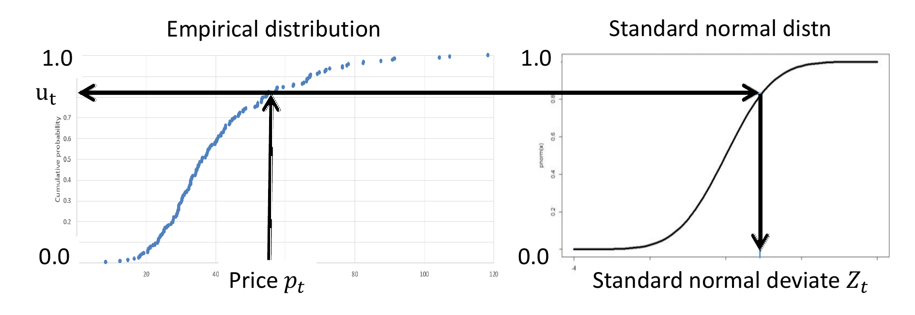
We can use this method to transform the highly non-normal prices $p_t$ to the sequence $z_t$ of values that are normally distributed with mean 0 and variance 1, where we can also capture correlations. We can then perform any time series modeling on the sequence $z_t$. After this, any estimates coming from this normalized model can be transformed back to prices by tracing the path in Figure 8.5 in the reverse direction: $u_t = \Phi(z_t)$, and then $p_t = F^{-1}_P(u_t)$.

This strategy is very effective when dealing with data that is not normally distributed, and performs much better than the jump diffusion model, which is popular in finance.

Designing policies

We are going to illustrate solving this problem using two classes of policies, plus a hybrid:

• Policy search – We are going to use a simple buy-low, sell-high parameterized policy. This belongs to the PFA class of policies (policy function approximations).
• Lookahead policy – We will use Bellman’s equation to produce a value function approximation that approximates the impact of a decision now on the future. This belongs to the VFA class of policies (policies based on value function approximations).
• Hybrid policy – Finally, we are going to introduce a tunable class of policy that begins with a policy based on value functions, and then switches to policy search to further tune the policy. This will start as a VFA policy, but then transition to a parametric cost function approximation (CFA) when we use policy search to tune the parameters of what started as the value function approximation.

Policies based on Bellman’s equation require computing (or approximating) the value $V_{t+1}(S_{t+1})$ which results from being in a state $S_t$, taking a decision $x_t$, and then observing random exogenous information $W_{t+1}$. We first saw these methods in the context of shortest path problems. One significant difference now is that the state $S_{t+1}$ is random given $S_t$ and $x_t$ (in the shortest path problem, only the cost $\chat_t$ was random). Also, our state variable now has two continuous dimensions, rather than just the discrete node.

We first describe the buy-low, sell-high policy, and then introduce three methods based on approximating Bellman’s equation:

• Classical backward dynamic programming, which produces an optimal policy.
• Backward approximate dynamic programming.
• Forward approximate dynamic programming.

We finish with a description of a hybrid policy that combines value function approximations from Bellman’s equation with a form of policy search.

Buy-low, sell-high

A buy-low, sell-high policy works on the simple principle of charging the battery when the price falls below a lower limit, and selling when the price goes above an upper limit. The policy can be written as

We now have to tune $\theta = (\theta^{buy}, \theta^{sell})$. We evaluate our policy by following a sample path of prices $p_t(\omega)$ (or we may be observing the changes in prices $\phat(\omega)$). Assuming we are generating sample paths from a mathematical model, we can generate sample paths $\omega^1, \ldots, \omega^N$. We can then simulate the performance of the policy over each sample path and take an average using

Tuning $\theta$ requires solving the problem

Since $\theta$ has only two dimensions, one strategy is to do a full grid search by discretizing each dimension, and then searching over all possible values of the two dimensions. A common discretization is to divide a region into 5-percent increments. Including the boundaries, this means we have to represent 21 values of each parameter, creating a grid of size 441 points, which is manageable (although not trivial) for most problems.

We note that a brute-force grid search only works if we run enough simulations $N$ so that the variance in the estimate $\Fbar^\pi(\theta)$ is relatively small. However, we have methods for doing the search for $\theta$ even with noisy estimates of the performance of the policy, as presented in Chapter 7.

We are going to see the optimization problem given by $\eqref{eq:buylowpolicysearch}$ repeatedly, since the simplest policies always feature tunable parameters. The problem $\eqref{eq:buylowpolicysearch}$ can be solved using derivative-based methods if we are able to compute (or approximate) derivatives of $\Fbar^{low-high}(\theta\vert S_0)$ with respect to $\theta$. When this is not possible, we have to use derivative-free methods, which is precisely the problem we faced in Chapter 2.

Backward dynamic programming

Backward dynamic programming involves directly solving Bellman’s equation

where $S_{t+1} = S^M(s_t,x_t,W_{t+1})$, and where the expectation is over the random variable $W_{t+1}$. Assume that $W_{t+1}$ is discrete, taking values in $\Wcal = {w_1, w_2, \ldots, W_M}$, and represent the probability distribution using

We write the distribution as depending on the state $s_t$ and decision $x_t$, but this depends on the problem. For example, we might reasonably assume that the change in the price $p_{t+1}-p_t$ depends on the current price $p_t$ (if prices are very high they are more likely to drop), which would be a reason to condition on $s_t$. We might even need the dependence on $x_t$ if purchasing a large quantity of electricity from the grid drives up prices.

We can then rewrite equation $\eqref{eq:energystoragebellman}$ as

A vanilla implementation of backward dynamic programming exhibits four loops:

1. The loop stepping backward in time from $T$ to time $0$.
2. The loop over all possible states $s_t\in\Scal$ (more precisely, this is the set of possible values of the state $S_t$ at time $t$).
3. The loop that would be required to search over all possible decisions $x_t$ in order to solve the maximization problem.
4. The loop over all possible values of the random variable $W$ that is captured in the summation required to compute $V_t(s)$.

It is useful to consider the range of values that each loop might take. For an energy problem, we might optimize a storage device in hourly increments over a day, giving us 24 time steps. If we use 5-minute time steps (some grid operators update prices every 5-minutes), then a 24 hour horizon would imply 288 time periods (multiply by seven if we want to plan over a week). If we are doing frequency regulation, then we have to make decisions every 2 seconds, which translates to 43,200 time periods over a day.

Our state variable consists of $S_t = (R_t,p_t)$, which means we have to replace the loop over all states, with nested loops over all values of $R_t$, and then all values of $p_t$. Since both are continuous, each will have to be discretized. The resource variable $R_t$ would have to be divided into increments based on how much we might charge or discharge in a single time increment. We then have to discretize the grid price $p_t$. Grid prices can go as low as -$100, and as high as $10,000 (in extreme cases). A reasonable strategy might be to construct an empirical distribution, and then represent prices corresponding to, say, each increment of two percent of the cumulative distribution, giving us 50 possible prices.

The number of charge-discharge decisions might be as small as three (charge, discharge or do nothing), or much larger if we can charge or discharge at different rates.

Finally, the probability distribution $f^W(w)$ would be the distribution of the random changes in prices, $\phat_{t+1}$. Again, we recommend constructing an empirical distribution of the changes in $\phat_{t+1}$ and then discretizing the cumulative distribution into increments of, say, two percent.

If we have a two-dimensional state variable (as is the case with our basic model), then we already have five loops (time, the two state variables, the max operator over $x$, and then the summation over outcomes of $W$). This can get expensive, and we have just started. Now imagine that we are using the time series model in equation $\eqref{eq:energytimeseriesmodel}$, where we now have to keep track of the prices $(p_t, p_{t-1}, p_{t-2})$. In this case, our state variable would be

In this case, we would now have seven nested loops. While the complexity depends on the discretization of the continuous variables, running this backward dynamic programming algorithm could easily require a year (or more).

Given how difficult it is to use Bellman’s equation, even for this relatively simple problem, it is surprising that this specific approach is still being taught in classes. Given the complexity, there has been extensive research into methods that approximate Bellman’s equation, which have been grouped under names like approximate dynamic programming and reinforcement learning. We are going to describe two strategies for approximating Bellman’s equation known as backward ADP and forward ADP.

Backward approximate dynamic programming

A powerful algorithmic strategy is known as “backward approximate dynamic programming.” This approach progresses exactly as we just did above, with one difference. Instead of looping over all the states, we choose a random sample $\Shat$. We then compute the value of being in state $s\in\Shat$ just as we originally did, and compute the corresponding value $\vhat$. Assume we repeat this $N$ times, and acquire a dataset $(\shat^n, \vhat^n), n=1, \ldots, N$. We then use this to fit a statistical model, such as the linear model given by:

where $\phi_f(s), f=1, \ldots, F$ is a set of appropriately chosen features. Examples of features might be

Note that with a constant term $\theta_0$, this model has only eight coefficients to be estimated. Sampling a few hundred states should be more than enough to get a good statistical approximation. This methodology is relatively insensitive to the number of state variables, and of course there is no problem if any of the variables are continuous.

A challenge whenever we use a parametric model such as the linear model above is that we have to specify the features $\phi_f(S_t)$. As neural networks became popular, researchers began to use this approach, including deep neural networks which might require estimating millions of parameters. The advantage of this approach is that it removes the need to specify the structure of the model, but the price is that you need far more observations. Deep neural networks offer the attractive property of being able to approximate any function, but this also means they may model noise. Neural networks also struggle to replicate known problem structure such as monotonicity (the bigger the inventory, the bigger the value) or convexity.

We have found backward ADP to work exceptionally well on a small set of problems (see Reinforcement Learning and Stochastic Optimization, Section 15.4, for a summary of comparisons of backward ADP against benchmarks), but there are no guarantees, and its performance clearly depends on choosing an effective set of features. In one application, we reduced a run time of 30 days for a standard backward MDP algorithm, down to 20 minutes, with a solution that was within 5 percent of the optimal (produced by the one-month run time). But again, there are no guarantees of this performance.

Forward approximate dynamic programming

Forward approximate dynamic programming works in an intuitive way. Imagine that we start with a value function approximation $\Vbar^{x,n-1}_t(S^x_t)$ around the post-decision state $S^x_t$ that we computed from the first $n-1$ iterations of our algorithm. We first introduced the idea of post-decision states in Chapter 1, but this is the state immediately after we make a decision, but before any new information has arrived.

Now, imagine that we are in a particular state $S^n_t$ during the $n$th iteration of our algorithm, following a sample path $\omega^n$ that guides the sampling as we step forward in time. Assume we have a function $S^{x,n}_t = S^{M,x}(S^n_t,x)$ that takes us to the post-decision state. For our energy problem where $S^n_t = (R^n_t,p^n_t)$, the post-decision state would be

We then make a decision using

Given $S^n_t$ and our decision $x^n_t$, we then sample $W_{t+1}(\omega^n)$ which translates to the change in the prices $\phat^n_{t+1}$. We then simulate our way to the next state

Thus, we are just simulating our way forward in time, which means we do not care how complex the state variable is. There are different strategies for then updating the value function approximation $\Vbar^{n-1}_t$:

This leaves the actual update in an updating function $U^V(\cdot)$ since this depends on how we are approximating the value function.

Forward approximate dynamic programming is attractive because it scales to high dimensional problems. At no time are we looping over all possible states or outcomes. In fact, we can even handle high dimensional decisions $x$ if we approximate the value function appropriately so that we can take advantage of powerful algorithms. However, forward ADP (as with backward ADP) possesses little in the way of performance guarantees.

A hybrid policy search-VFA policy

Whatever way we choose to approximate the value function, our policy is given by

We simulate the policy forward, where we let $\omega^n$ represent a sample path of the exogenous information (that is, the set of changes in prices). It is frequently the case that we are going to test our policy on historical data, in which case there is only a single sample path. However, if we have developed a mathematical model of the uncertain prices, we can create a sample path $\omega$ that we use to approximate the value of a policy (we could also create multiple sample paths and take an average):

This means that the method is well suited to approximating even high-dimensional problems that might arise in logistics.

When we are building a value function approximation (which belongs in the lookahead class of policies), we typically no longer have a step where we tune the policy. However, this does not mean that we cannot try. Assume that our value function is given by the linear model in equation $\eqref{eq:energylinearvfa}$. We can now write our policy using

It makes sense to use one of our backward or forward ADP algorithms to get an initial estimate of $\theta$, but as we noted above, there is no guarantee that the resulting policy is high quality. However, we can always make it better by using this as a starting point,

Now, we just have to solve the policy search problem that we might pose as

In our earlier examples for policy search, $\theta$ was a scalar, which makes this problem relatively easy. Now, $\theta$ is a vector which might have dozens of dimensions. We are going to return to this problem later.

Some cautionary notes about ADP

We have used this problem setting to provide a relatively in-depth tour of methods that are based on the idea of approximating the value of being in a state. This has been studied under terms such as “approximate dynamic programming” or “reinforcement learning.” These methods have attracted considerable attention from the academic research communities, but in practice, the methods are not easy. Sequential decision problems are everywhere, but successful applications in practice are relatively rare.

Lookup table approximations, where we estimate the value for each discrete (or discretized) state, do not scale when the state variable has more than three dimensions. Using approximation strategies such as our linear approximation typically does not work since these approximations have to be globally accurate, since we may visit any state. At the same time, local approximations (which are forms of nonparametric models) can struggle because the flexibility of local approximations introduces instability.

Complicating the process is that we depend on our approximate value function to make decisions, which creates a vicious cycle. Our initial approximations are not very good, and as a result lead to bad decisions. These bad decisions are then used to update the value function approximation, and from there you can see the downward spiral.

The idea of tuning a value function approximation, as we did in equation $\eqref{eq:optthetavfa}$, is promising because it directly optimizes the performance of the policy. Oddly, this idea is not widely used. We just note that tuning $\theta$ using these simulations is not easy. So, we urge caution to any reader who decides to try these approaches.

What did we learn?

• We revisit a simple inventory problem from Chapter 1, but in the context of energy storage, with both physical and informational variables.
• We describe a variety of stochastic models for electricity prices to illustrate the richness of uncertainty modeling.
• We describe a range of policies: a PFA (buy-low, sell-high), a VFA policy (based on backward approximate dynamic programming) as well as forward approximate dynamic programming.
• Finally, we introduce the idea of estimating a linear model for a value function approximation using the techniques of approximate dynamic programming, and then perform direct policy search on the coefficients of the linear model. So, this is a VFA-based policy initially, and then turns into a form of CFA policy with a parameterized objective function.

Exercises

Review questions

1. Given the heavy-tailed nature of electricity prices, what is wrong with using a time-series model?
2. Briefly sketch how we separate the prices that fall within normal variations (three standard deviations) from the more extreme observations.
3. Using historical data to fit an empirical distribution should give us a probability distribution that matches history. What other errors might still be present in the stochastic model of prices?
4. Describe in words what the transformation of the data in the hybrid time-series section is accomplishing.
5. Classical backward dynamic programming quickly blows up from the curse of dimensionality. Describe in words how backward approximate dynamic programming overcomes the curse of dimensionality. For example, if we were to double the number of dimensions in the state variable, describe how this complicates backward ADP.

Problem solving questions

1. Write out the five elements of the basic model for the energy storage problem as they are given in the text. Write out the objective function assuming that the policy is the buy-low, sell-high policy $$ X^{low-high}(S_t\vert \theta) = \begin{cases} -1 & \text{if } p_t < \theta^{buy}, \\ 0 & \text{if } \theta^{buy} \leq p_t \leq \theta^{sell}, \\ +1 & \text{if } p_t > \theta^{sell}. \end{cases} $$ Write the objective function in terms of searching over the parameters of the policy. Also, write the expectation in the objective function using the nested form that reflects each random variable.
2. In the section on modeling uncertainty, we introduce a time series model for prices given by $$ p_{t+1} = \thetabar_{t0} p_t + \thetabar_{t1} p_{t-1} + \thetabar_{t2} p_{t-2} + \varepsilon_{t+1}. $$ The book describes the updating equations for the coefficient vector $\thetabar_t = (\thetabar_{t0},\thetabar_{t1}, \thetabar_{t2})$. Remembering that the state $S_t$ consists of *all* the information needed to model the system from time $t$ onward, give the updated state variable and transition function to handle this price process.

Programming questions

These exercises use the Python module EnergyStorage_I on tinyurl.com/sdagithub.

1. Using the python module run a grid search for the parameter vector $\theta = (\theta^{buy}, \theta^{sell})$ by varying $\theta^{sell}$ over the range from 1.0 to 100.0 in increments of \$1 for prices, and varying $\theta^{buy}$ over the range from 1.0 to $\theta^{sell}$, also in increments of \$1. The prices will be actual historical hourly prices for an 8 day period.
2. Solve for an optimal policy by using the backward dynamic programming strategy described above (the algorithm has already been implemented in the python module). Assume that the price process evolves according to $$ p_{t+1} = p_t + \varepsilon_{t+1}, $$ where $\varepsilon_{t+1}$ follows an empirical distribution based on the price differences of the actual historical prices.
   1. Run the algorithm where prices are discretized in increments of \$1, then \$0.50 and finally \$0.25. Compute the size of the state space for each of the three levels of discretization, and plot the run times against the size of the state space.
   2. Using the optimal value function for the discretization of \$1 and compare the performance against the best buy-sell policy you found in part (a).
3. Download the spreadsheet "Chapter8_electricity_prices" from [tinyurl.com/sdamodelingsupplements](https://tinyurl.com/sdamodelingsupplements/). Use the data in the tab "electricity prices" for the following questions:
   1. Build an empirical cumulative distribution $F_P(p) = Prob[P \leq p]$ where $P$ is a randomly chosen price for a particular hour over the one-week period in the dataset.
   2. Let $F^{-1}_P(u)$ be the inverse cumulative distribution, where $u$ is between 0 and 1. Find the price $p(u) = F^{-1}_P(u)$ corresponding to $u = 0, 0.1, 0.2, \ldots, 0.9, 1.0$. Giving each of these prices a probability of 1/11, find the cumulative distribution, and compare it to the cumulative distribution that you created in part (a). Do these appear to match?
4. Using the spreadsheet "Chapter8_electricity_prices," fit a mean reversion model of the form $$ \begin{align} p_{t+1} = p_t + \beta (\mubar_t - p_t) + \varepsilon_{t+1} \label{eq:priceexercise} \end{align} $$ where $$ \mubar_t = (1-\alpha)\mubar_{t-1} + \alpha p_t. $$ Assume $\alpha = 0.15$. Find $\beta$ that minimizes $$ G(\beta) = \sum_{t=0}^T \big(p_{t+1} - (p_t + \beta (\mubar^t-p_t))\big)^2. $$
   1. Fit the mean reversion model by doing a simple one-dimensional search (e.g. try values between 0 and 1 in increments of 0.1).
   2. Compute the standard deviation $\sigma$ of $\varepsilon$ from your sample (we assume the mean is 0). Note that we assume there is a single, constant standard deviation, although we allow the mean $\mubar_t$ to vary over time.
   3. Using the value of $\beta$ you found in (a), generate 10 sample paths using equation $\eqref{eq:priceexercise}$ by sampling $\varepsilon_{t+1}$ from a normal distribution with mean 0 and standard deviation $\sigma$. Plot the sample paths in a graph, and compare the behavior of your sample paths to the historical prices. Do they seem similar?
5. Now you are going to fit a jump diffusion model which is given by $$ p_{t+1} = p_t + \beta(\mubar_t - p_t) + \varepsilon_{t+1} + J_{t+1} \varepsilon_{t+1}, $$ where $J_{t+1} = 1$ with some jump probability (that we calculate below) and 0 otherwise, and $\varepsilon^J_{t+1}$ is the random size of the jump when they happen. Follow the steps below to fit the jump diffusion model and compare the results to history.
   1. Using the value of $\beta$ from exercise 11, pass over the data and identify all the data points that fall outside of the range $[\mubar_t \pm 3 \sigma]$.
   2. Using the same value of $\beta$ you found in exercise 11, run the mean reversion over the data a second time, but this time only include the data points that were not excluded in part (a). Find the new mean and standard deviation of $\sigma$ on the data that was not excluded.
   3. Repeat (b) one more time on the datapoints that were retained, again excluding data points outside the $\pm 3 \sigma$ range.
   4. Compute the probability of a jump as the fraction of points that were excluded by the time you finish part (c) (by now you have run the process of excluding datapoints twice). Also, compute the mean and standard deviation of the points that were excluded.
   5. Now, run 10 simulations of your jump diffusion model, using the final mean and variance for the retained and excluded points, and where you sample jumps using the jump diffusion probability. Compare these simulations to history, and discuss whether the resulting price paths are more realistic than what you found in exercise 11, and compare the price paths to actual history.
6. We are going to try again to get a good fit of the prices by repeating parts of exercises 11 and 12 using transformed prices.
   1. Using the cumulative distribution from exercise 10, convert each of the prices to a uniformly distributed random variable using the identity $U_t = F_P(p_t)$.
   2. Next convert your uniformly distributed random variables $U_t$ into normally distributed random variables with mean 0 and variance 1 using $Z_t = \Phi^{-1}(U_t)$ where $\Phi(z)$ is the cumulative distribution of the standard normal distribution, and $\Phi^{-1}(U_t)$ is the inverse of this distribution. This is captured by the norm.s.inv(p) function in Excel, which returns the $Z$ value corresponding to a probability $p$ (which is given by the variable $U_t$).
   3. We now have to refit $\beta$ in the mean reversion equation from exercise 11. This time, instead of using the price $p_t$, we use the normalized quantity $Z_t$; otherwise everything is the same (so you can just follow the process when you fit $\beta$ for the raw prices).
   4. Now use your model from (c) (with the new value for $\beta$) to create a sample path of $Z_t$ values. Then, use $U_t = \text{norm.s.dist}(Z_t,1)$ to get the probability that $Z_t \leq z$ (which is uniformly distributed between 0 and 1). Finally, map the $U_t$ value back to a price using the cumulative distribution you found in exercise 11. Plot one sample path (this is not too hard if you are proficient in Excel — otherwise the painful part is this last step).
   5. Compare the behavior of the resulting sample path to the historical distribution. Note that the distribution of prices should be perfect, but the series of prices may still not look like a good fit. What mistakes might we still be making?