Chapter 12: Ad-click optimization

Chapter overview

This chapter addresses the problem of optimizing the policy for placing bids to maximize returns on e-commerce platforms such as Google and Facebook. These platforms run sophisticated auctions to ensure that they are getting paid the full market value for the ads they display. The model of the problem, and the design of policies, is complicated by the need to represent three forms of uncertainty: the probability we win the bid we make on an ad, the outcome of whether or not we win the bid, and the revenue earned from winning the bid.

We explore three policies. The first two are relatively simple: a greedy policy that chooses the best bid given our current estimates of all uncertain quantities, and a randomized version of the greedy policy that encourages exploration. The third is more sophisticated: known as the “knowledge gradient” it maximizes the value of information from placing a particular bid. This requires finding an expectation of the improvement from what we learn from a given bid. The knowledge gradient involves relatively sophisticated probability calculations.

Narrative

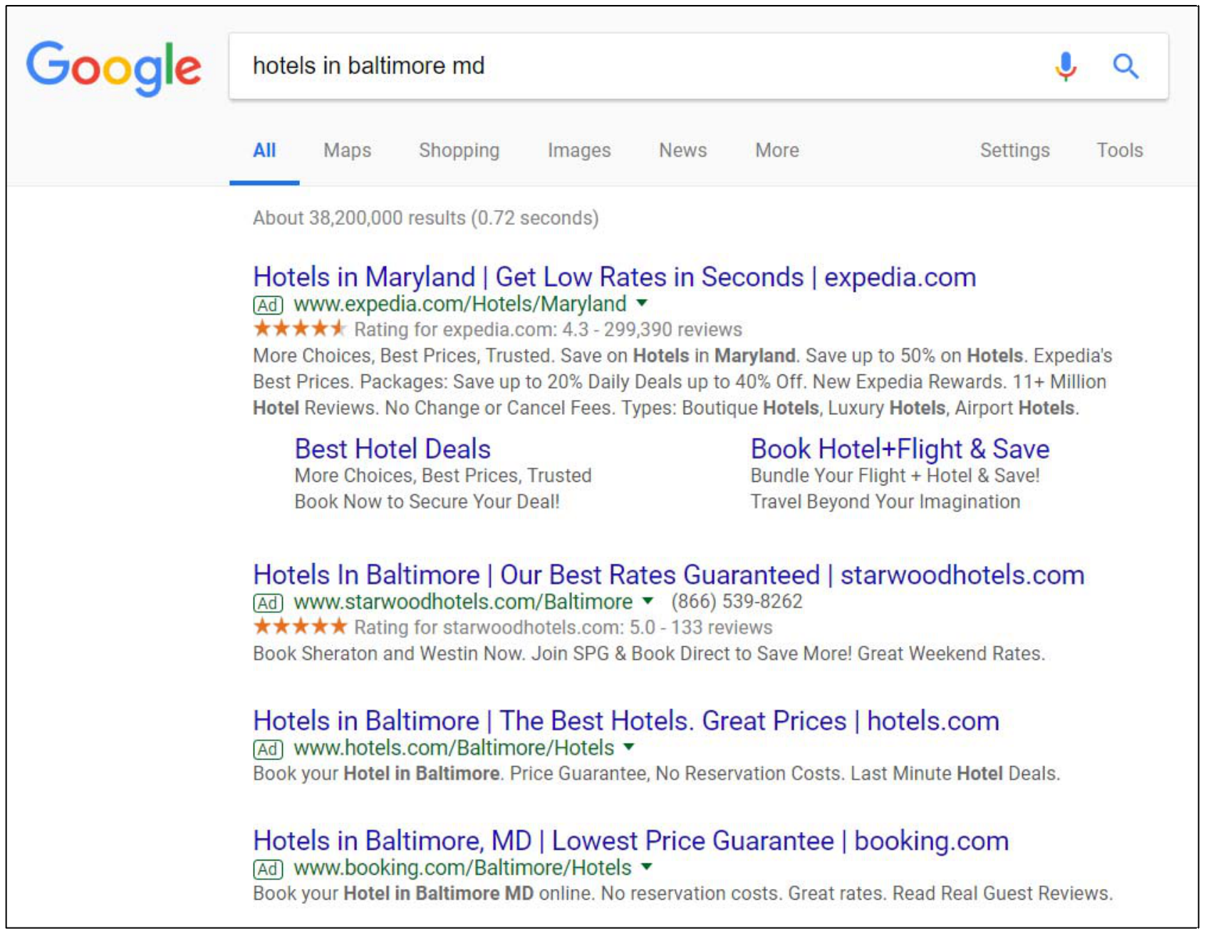
Companies advertising on internet sites such as Google have to bid to get their ads in a visible position (that is, at the top of the list of sponsored ads). When a customer enters a search term, Google identifies all the bidders who have listed the same (or similar) search terms in their list of ad-words. Google then takes all the matches, and sorts them in terms of how much each participant has bid, and runs an auction. The higher the bid, the more likely your ad will be placed near the top of the list of sponsored ads, which increases the probability of a click. Figure 12.1 is an example of what is produced after entering the search terms “hotels in baltimore md.”

If a customer clicks on the ad, there is an expected return that reflects the average amount a customer spends when they visit the website of the company. The problem is that we do not know the bid response curve. Figure 12.2 reflects a family of possible response curves. Our challenge is to try out different bids to learn which curve is correct.

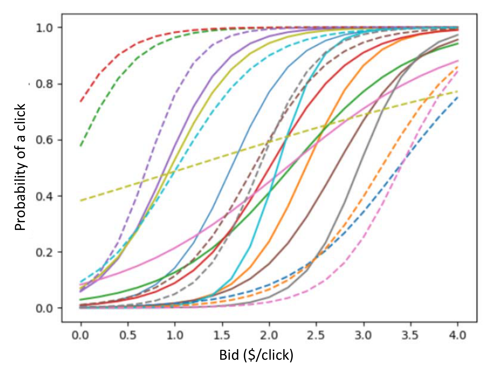
We begin by assuming that we can adjust the bid after every auction, which means we only learn a single response (the customer did or did not click on the link). It is possible that the customer looked at a displayed link and decided not to click it, or our bid may have been so low that we were not even in the list of displayed ads.

Our challenge is to design a policy for setting the bids. The goal is to maximize the net revenue, including what we make from selling our products or services, minus what we spend on ad-clicks.

Framing the problem

The answers to our three framing questions are:

• Metrics: Maximize the expected net revenue from selling products that are advertised on the platform, minus the amount paid to run the ad.
• Decisions: How much to bid for the ad.
• Uncertainties: Whether a bid is successful, and the amount of revenue received from a successful bid.

Basic model

We are going to assume that we use some sort of parameterized model to capture the probability that a customer clicks on an ad. At a minimum this probability will depend on how much we bid for an ad – the more we bid, the higher the ad will appear in the sponsored ad list, which increases the likelihood that a customer will click on it. Let $K^n = 1$ if the $n$th customer clicks on the ad. Let

where $Prob[K^{n+1}=1\vert \theta=\theta_k,x]$ will be described by a logistic function given by

This function is parameterized by $\theta = (\theta^{const}, \theta^{bid})$. We do not know what $\theta$ is, but we are going to assume that it is one of a sampled set $\Theta = {\theta_1, \ldots,\theta_K}$.

State variables

The initial state $S^0$ includes $\Theta = {\theta_1, \ldots, \theta_K}$, the set of possible values that $\theta$ may take; and $\Rbar^0$, the initial estimate of revenue earned when a customer clicks on a link.

The dynamic state variables $S^n$ include $p^n_k$, the probability that the true $\theta = \theta_k$, with $p^n = (p^n_k)_{k=1}^K$; and $\Rbar^n$, the estimate of revenue earned from an ad-click after $n$ auctions.

Our dynamic state variable, then, is

Note that we can create a point estimate of $\theta$ after $n$ observations using

but this is a statistic that we can compute from the information in $S^n$, so we do not put $\thetabar^n$ in the state variable.

Decision variables

Our only decision variable is the bid which we define as $x^n$, the bid (in $ per click) for the $(n+1)$st auction. As before, we let $X^\pi(S^n)$ be our generic policy that gives us the bid $x^n$ as a function of the information available to us, represented by $S^n$, which means that we would write

We assume that the policy enforces any constraints, such as making sure that the bid is not negative or something too large.

Exogenous information

In our initial model, we only observe the results of a single auction, which we model using:

and $\Rhat^{n+1}$, the revenue earned from the $n+1$st auction. This means our complete exogenous information variable is

Transition function

The transition function for this problem will seem a lot more complicated than others in this volume, which is because we are updating beliefs about the uncertainty in the parameter vector $\theta$. We need to emphasize that all the transition equations can be coded relatively easily.

We are going to update our estimated revenue when a customer clicks on the ad using:

Thus, we only update our estimated revenue when we get a click. The parameter $\alpha^{lrn}$ is a smoothing parameter (sometimes called a “learning rate”) between 0 and 1 that we fix in advance.

We next address the updating of the probabilities $p^n_k$. We let $H^n$ be the history of states, decisions and exogenous information

We use this to write

The way to read the conditioning on the history $H^n$ is “$p^n_k$ is the probability $\theta = \theta_k$ given what we know after $n$ observations.” We then use Bayes theorem to write

Remember that the history $H^n$ includes the decision $x^n$ which, given a policy for making these decisions, is directly a function of the state $S^n$ (which in turn is a function of the history $H^n$). We now use our logistic curve in equation $\eqref{eq:adclicklogisticregression}$ to write

We then note that

Finally, we note that the denominator can be computed using

Our use of a sampled representation of the possible outcomes of $\theta$ is saving us here. Even if $\theta$ has only two dimensions (as it is here, but only for now), performing a two-dimensional integral over a multivariate distribution for $\theta$ would be problematic.

Equations $\eqref{eq:adclicktransition2a}$–$\eqref{eq:adclicktransition2c}$ allow us to calculate our Bayesian updating equation for the probabilities in $\eqref{eq:adclicktransition2}$. Equations $\eqref{eq:adclicktransition1}$–$\eqref{eq:adclicktransition2}$ make up our transition function

Objective function

We begin by writing the single period profit function as

which means we make nothing if the customer does not click on the ad ($K^{n+1} = 0$). If the customer does click on the ad ($K^{n+1} = 1$), we receive revenue given by $\Rhat^{n+1}$, but we also have to pay what we bid for the ad-click, given by our bid $x^n$.

We will end up taking the expected contribution, which we write as

There are three random variables hidden in the expectation:

• $\theta$, with distribution $p^n = (p^n_1, \ldots, p^n_K)$ (contained in $S^n$).
• $K^{n+1}$, where $P^{click}(\theta,x) = Prob[K^{n+1}=1\vert \theta,x]$.
• $\Rhat^{n+1}$, which we observe from some unknown distribution if $K^{n+1}=1$, and where $\Rhat^{n+1}=0$ if $K^{n+1}=0$ (we do not get any revenue if the customer does not click on the ad).

We can then break the expectation into three nested expectations:

We start by taking the expectation over $\Rhat$ where we just use $\E {\Rhat^{n+1}\vert S^n} = \Rbar^n$ (remember that $\Rbar^n$ is in the state variable $S^n$), which allows us to write

Next we are going to take the expectation over $K^{n+1}$ for a given $\theta$ using

where we have used the fact that $(\Rbar^n - x^n) K^{n+1}=0$ if $K^{n+1}=0$.

Finally we take the expectation over $\theta$ using

We are going to let $\Cbar(S^n,x)$ be the expected contribution, which is to say

Our objective function can now be written as

Note that the conditioning on $S_0$ is how we communicate our prior $p^0_k = Prob[\theta=\theta_k]$ to the model. As before, we would approximate the expectation by averaging over simulated samples of the true value of $\theta$, and the observed clicks $K^n$ and revenues $R^n$.

Modeling uncertainty

We have three forms of uncertainty: the ad-click $K^{n+1}$, the revenue we receive $\Rhat^{n+1}$ if $K^{n+1}=1$, and then the true value of $\theta$. We are going to assume that we simply observe $\Rhat^{n+1}$ from a real datastream, which means we do not need a formal probability model for these random variables. We assume that $K^{n+1}$ is described by our logistic function

but it is important to recognize that this is just a fitted curve. The values of $K^{n+1}$ are observed from data, which means we have no guarantee that the distribution precisely matches our logistic regression.

Finally, we assume that $\theta \in \Theta = {\theta_1, \ldots, \theta_K}$ which is also an approximation. There are ways to relax the requirement of a sampled set, but the logic becomes somewhat more complicated without adding much educational value.

Designing policies

We are going to explore three policies for learning:

• Pure exploitation – Here we always place the bid that appears to be the best given our current estimates.
• An excitation policy – We introduce exploration into our exploitation policy by adding in a random noise term which forces the system to explore in regions near the areas we think are best (this is popular in engineering where states and decisions are continuous).
• A value of information policy – We are going to maximize the value of information from placing a bid and learning the outcome.

Pure exploitation

The starting point of any online policy should be pure exploitation, which means doing the best that we can. To compute this we start by using

To find the best bid, we find (after a bit of algebra) the derivative with respect to the bid $x$

where

Now we want to find the bid $x^\ast $ where

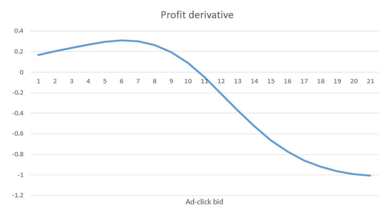
Figure 12.3 shows $\frac{d \Cbar(x\vert \theta)}{d x}$ versus the bid $x$, showing the behavior that it starts positive and transitions to negative. The point where it is equal to zero would be the optimal bid, a point which can be found numerically quite easily. Let $X^{explt}(S^n)$ be the bid $x^\ast $ satisfying $d \Cbar(x)/dx = 0$.

This means that we have to run a numerical algorithm to compute the policy. This is a greedy policy which falls in the CFA class, but without any tunable parameters.

An excitation policy

A potential limitation of our pure exploitation policy is that it ignores the value of trying a wider range of bids to help with the process of learning the correct values of $\theta$. A popular strategy is to add a noise term, known in engineering as “excitation,” giving us the policy

where $\varepsilon(\rho) \sim N(0,\rho^2)$. In this policy, $\rho$ is our tunable parameter which controls the amount of exploration in the policy. If it is too small, then there may not be enough exploration. If it is too large, then we will choose bids that are far from optimal, possibly without any benefit from learning.

A value of information policy

The pure exploitation and excitation policies we just introduced are both relatively simple. Now we are going to consider a policy that maximizes the value of information in the future. This seems like a reasonable idea, but it requires that we think about how information now affects what decision we might make in the future, and this will be a bit more difficult.

Our exploitation policy assumes that the estimated parameters $\theta^n$ after $n$ experiments is the correct value, and chooses a bid based on this estimate. Now imagine that we bid $x^n=x$ and observe $K^{n+1}$ and $\Rhat^{n+1}$, and use this information to get an updated estimate of $\theta^{n+1}$ as well as $\Rbar^{n+1}$. We can then use these updated estimates to make a better decision. We want to choose the bid $x$ that gives us the greatest improvement in the value of information from a decision, recognizing that we do not know the outcome of $W^{n+1} = (\Rhat^{n+1},K^{n+1})$ until we actually place the bid.

Let $\theta^{n+1}(x^n,W^{n+1})$ be the updated estimate of $\theta$ assuming we bid $x^n=x$ and observe $W^{n+1} = (\Rhat^{n+1},K^{n+1})$. This is a random variable, because we are thinking about placing a bid $x^n=x$ for the $n+1$st auction, but we have not yet placed the bid, which means we have not yet observed $W^{n+1}$.

To simplify our analysis, we are going to assume that the random variable $K^{n+1} = 1$ with probability $P^{click}(\theta,x)$ and $K^{n+1} = 0$ with probability $1-P^{click}(\theta,x)$. We are then going to assume that our estimate of the revenue we receive from an ad-click has stabilized, which means that $\Rbar^{n+1} \approx \Rbar^n$.

We can think of this as an approximate lookahead model, where $\Rbar^n$ does not change. We would then write our exogenous information in our lookahead model as

where the double-superscript $(n,n+1)$ means that this is the information in a lookahead model created at time $n$, looking at what might happen at time $n+1$. The random variable $\Ktilde^{n,n+1}$ is the ad-click that we are simulating might happen in our lookahead model, rather than the actual observation of whether someone clicked on the ad. Just remember that we use tilde for any variable in our lookahead model, and these variables will be indexed by $n$ (the time at which we are initiating the lookahead model), and $n+1$ (since we are looking one time period forward in the lookahead model).

We next use our updating equation $\eqref{eq:adclicktransition2}$ for the probabilities $p^n_k = Prob[\theta=\theta_k\vert H^n]$. We can write these updated probabilities as $\ptilde^{n,n+1}_k(\Ktilde^{n,n+1})$ to capture the dependence of the updating on $\Ktilde^{n,n+1}$ (equation $\eqref{eq:adclicktransition2}$ is written for $\Ktilde^{n,n+1}=1$). Since $\Ktilde^{n,n+1}$ can take on two outcomes (0 or 1) we will have two possible values for $\ptilde^{n,n+1}_k(\Ktilde^{n,n+1})$.

Now imagine that we perform our pure exploitation policy $X^{explt}(S^n\vert \theta^n)$ that we described above, but we are going to do it in our approximate lookahead model (this is where we ignore changes in $\Rbar^n$). Let $\Stilde^{n,n+1}$ represent our state in the lookahead model given by

Remember – since $\Ktilde^{n,n+1}$ is a random variable (we are still at time $n$), $\Stilde^{n,n+1}(\Ktilde^{n,n+1})$ is also a random variable, which is why we write its explicit dependence on the outcome $\Ktilde^{n,n+1}$.

The way to think about this lookahead model is as if you are playing a game (such as chess) where you think about a move (for us, that would be the bid $x^n$) and then, before you make the move, think about what might happen in the future. In this problem, our future only has two outcomes (whether or not a customer clicks on the ad), which means two possible values of $\Stilde^{n,n+1}$, which produce two sets of updated probabilities $\ptilde^{n,n+1}(K^{n+1})$.

Finally, this means that there will be two values of the optimal myopic bid (using our pure exploitation policy) $X^{explt}(\Stilde^{n,n+1})$. The expected contribution we would make in the future is then given by $\Ctilde(\Stilde^{n,n+1},\xtilde^{n,n+1})$ where $\xtilde^{n,n+1}$ (this is the decision we are thinking of making in the future) is given by

This means there are two possible optimal decisions, which means two different values of the expected contribution $\Ctilde(\Stilde^{n,n+1},X^{explt}(\Stilde^{n,n+1}))$. For compactness, let’s call these $\Ctilde^{n,n+1}(1)$ (if $\Ktilde^{n,n+1} = 1$) and $\Ctilde^{n,n+1}(0)$ (if $\Ktilde^{n,n+1} = 0$). Think of these as the expected contributions that might happen in the future given what we know now. Finally we can take the expectation over $\Ktilde^{n,n+1}$ to obtain the expected contribution of placing a bid $x^n=x$ right now, which we can compute using

Our policy, then, is to pick the bid $x$ that maximizes $\Cbar^n(x)$. Assume that we discretize our bids into a set $\Xcal = {x_1, \ldots, x_M}$. Our value of information policy would be written as

We note that this is a direct lookahead approximation (DLA) class of policy.

Value of information policies are quite powerful. They are harder to compute, but do not have any tunable parameters. Imagine, for example, doing this computation when there is more than two outcomes. For example, if we had not made our simplification of holding $\Rbar^n$ constant, we would have to recognize that this state variable is also changing.

We note only in passing that we have run many comparisons of different learning policies, and the one-step lookahead value of information often works quite well. We used this setting because it made the derivations much simpler.

A word of caution is in order. Learning problems where the outcome is 0 or 1 are problems where a single experiment provides very little information. Instead, it is better to assume that we make our decision (that is, set the bid) and then observe it for, say, $M$ auctions. This means that $\Ktilde^{n,n+1}$ might now be a number between 0 and $M$. The number $M$ becomes a tunable parameter, and the calculations just became a little more complex (we have to sum over $M+1$ realizations rather than just two), but this approach can work quite well.

Extension: Customers with simple attributes

Assume that we know the location of a customer down to a region or the nearest major city, which we designate by $L$. If we think that the behavior of each region is different, we could index $\theta$ by $\theta_\ell$ if the customer is from location $L=\ell$. This means that if there are 1,000 locations, then we have to estimate 1,000 models, which means 1,000 values of $\theta = (\theta^{const},\theta^{bid})$.

An alternative approach would be to specify a model of the form

where we are now going to use as our utility function

This is a more compact model because we now assume that the constant term $\theta^{const}$ and bid coefficient $\theta^{bid}$ do not depend on the location. Instead, we are just adding a shift $\theta^{loc}\ell$. So, we still have 1,000 parameters to estimate (the location coefficients), but before we had 2,000 parameters to estimate – $\theta^{const}\ell$ and $\theta^{bid}_\ell$ for each location $\ell \in {1, \ldots, L}$.

What did we learn?

• This is another pure learning problem (our diabetes problem in Chapter 4 was a pure learning problem) but this time we are using a nonlinear belief model, with a sampled model for the unknown parameter $\theta$ that determines the response to price.
• The transition function includes the Bayesian updating of the beliefs about the probabilities $p^n_k$ that the unknown parameter $\theta$ is equal to a specific value $\theta_k$.
• There are three forms of uncertainty: whether someone will click on an ad given the bid price; the revenue earned from clicking on the ad (for example, did the customer purchase the product), and the uncertainty about the market response captured by the unknown parameter $\theta$.
• We illustrate a pure exploitation policy, an excitation policy (which simply randomizes the recommended price from the exploitation policy), and a knowledge gradient policy that maximizes the value of information.

Exercises

Review questions

1. What probabilistic model is assumed for the random variable $K^n$ giving whether a customer clicked on the ad or not?
2. What probabilistic model did we assume for the unknown (and therefore uncertain) parameter vector $\theta$?
3. What probability distribution did we assume for the revenue $\Rhat^{n+1}$ we receive when the customer clicks on an ad?
4. Give the equation numbers of the equations that make up the transition function.
5. What probabilistic information is in the initial state $S^0$?
6. What is accomplished by adding the noise term $\varepsilon(\rho)$ to create the excitation policy? What specific parameter(s) does this help us identify?
7. Describe in words the logic behind the value of information policy. What is the value if learning whether or not a customer clicks on the ad does not change what we are going to bid?

Problem solving questions

1. Recommender system part I - Belief model - You are going to help design a recommender system that recommends products to advertise when a customer is scrolling through a website. Since the customer has to sign in, we can identify the $n$th customer by a vector of attributes $a=a^n$ that includes: $a_1$, gender (2 types); $a_2$, age range $(0$–$10, 11$–$20, \ldots, 70$–$100)$ (8 types); $a_3$, device type (smartphone, laptop, tablet) (3 types); $a_4$, region (200); and $a_5$, unique ID (email address) (100 million). Imagine that we are recommending text articles. Assume that the article we recommend for the $n$th customer has attributes $b=b^n$ that includes: $b_1$, news, sports, arts, business, cooking, real-estate (6 types); $b_2$, subcategory: if news, then international, national (by country), regional (region within a country); if sports, then by sport, and then by team (or athlete); and so on (a total of 500); $b_3$, source (website, newspaper, ...) (5 sources); $b_4$, author (2,000); and $b_5$, unique ID for article (6 million). We would like to estimate $P(b^n\vert a^n)$, the probability that the $n$th customer with attribute $a^n$ clicks on the link of an article with attribute $b^n$. When customer $a^n$ arrives, we are going to assume that we have to choose a news article from a set $\Bcal^n$, which is the set of articles available when the $n$th customer arrives (this set changes over time). We would like to choose an article with attribute $b\in\Bcal^n$ that maximizes the probability that our customer will click on this news article. Our policy has to choose a particular article with attribute $b^n$. Ideally, we want $P(b^n_5\vert a^n_5)$ which is the probability that user $a^n_5$ would select article $b^n_5$, but there are too many users and too many articles to get reasonable estimates of this probability. If we only consider the elements $a_1, a_2, a_3$ and $a_4$, there would be 9,600 combinations, with an average of approximately 10,000 people for each of these first four elements. Below, we are going to assume we just use $a_1$ and $a_2$, which means 16 types of people. We are going to create a set of features $\Fcal$ which are constructed from the elements of $a$ and $b$ that we wish to consider. We are just going to use the elements $\{a_1,a_2,b_1,b_2,b_3\}$ from which we are going to construct a set of feature variables $\phi_f(a,b),~f\in\Fcal$. Since these five elements are all categorical, the most elementary features are indicator variables. For example, for the gender attribute $a_1$ we have two genders from which we create two features: $$ \phi_{male}(a) = \begin{cases} 1 & \text{if } a_1 = male, \\ 0 & \text{otherwise.} \end{cases} \qquad \phi_{female}(a) = \begin{cases} 1 & \text{if } a_1 = female, \\ 0 & \text{otherwise.} \end{cases} $$ If we restrict ourselves to these elementary features, we would have one feature for each possible value for each element of the attributes $a_1,a_2,b_1,b_2,b_3$. Our process begins when the first customer logs in with attribute vector $a^1$, at which point we have to decide the attributes of an article $b^1$ to display to this user, and then observe $Y^1$, where $Y^1 = 1$ if the customer clicks on the article or 0 otherwise. This information is used to create an updated state $S^1$, after which we observe customer $a^2$. If $a^n$ is the attributes of the $n$th customer, then our decision is to choose $b^n$ using what we know, which we designate by $S^n$. Our goal is to model this problem and design a policy $B^\pi(S^n)$ that determines $b^n$. Our first challenge is to develop a belief model:
   1. If we use a lookup table belief model for $P(b\vert a)$ using the attributes $\{a_1,a_2, b_1,b_2,b_3\}$, how many parameters are we trying to estimate?
   2. Instead, consider using a logistic regression. First define a utility function $$ U(a,b\vert \theta) = \sum_{f\in\Fcal} \theta_f \phi_f(b\vert a), $$ where $\Fcal$ is the set of elementary features that we can construct from the elements $\{a_1,a_2,b_1,b_2,b_3\}$. Now create a logistic regression model for the probability of clicking on an article using $$ P(Y=1\vert a,b,\theta) = \frac{e^{U(a,b\vert \theta)}}{1+e^{U(a,b\vert \theta)}}. $$ What is the dimensionality of the vector $\theta$ assuming that we just use elementary indicator variables?
   3. Recognizing that the number of parameters in the parametric model in part (b) is much smaller than the number of parameters in the lookup table model in part (a), why would anyone use a lookup table belief model instead of a parametric model such as the logistic regression? Discuss the pros and cons of each type of belief model.
   4. We now need to estimate $\theta$. Assume we generate a sample of possible values of the vector $\theta$ which we represent as $\{\theta_1, \ldots, \theta_k, \ldots, \theta_K\}$, where each $\theta_k$ is a vector with element $\theta_{kf},~f\in\Fcal$. Start with the prior probability $p^0_k = 1/K$. Next assume that we observe the attributes of the first customer $a^1$, and then we make the decision to display an article with attribute $b^1$ (this is our decision variable). Assuming you know $p^n_k$, write out Bayes theorem to compute $p^{n+1}_k$ after observing a customer with attribute $a^{n+1}$, and then choosing an article with attribute $b^{n+1}$ after which you observe the outcome $Y^{n+1} = 1$.
2. Recommender system part II - System model - Now we are going to model all five elements of the problem.
   1. Give the elements of the pre-decision state $S^n$ and the post-decision state $S^{b,n}$.
   2. There are two forms of exogenous information in this process. What are they?
   3. Write out the sequence of states (pre- and post-), decisions and the different forms of exogenous information starting with what you know at time 0 and proceeding up to (but excluding) the arrival of the third customer. Write them in the order that they occur, with proper indexing (e.g. $n$ versus $n+1$).
   4. Write out the equations representing the transition function.
   5. Write out the objective function to find the best policy $B^\pi(S^n)$ (without specifying the type of policy).
3. Recommender system part III - Policy design - Finally we are going to try to design policies. Assume that we have $K=20$ possible values of $\theta$.
   1. Begin by assuming that we know that $\theta = \theta_k$. Write out a pure exploitation policy where we choose the attribute $b\in\Bcal^n$ that maximizes the probability of being chosen, given that $\theta = \theta_k$.
   2. Next assume that we do not know that $\theta=\theta_k$. Instead, $\theta=\theta_k$ with probability $p^n_k$. Rewrite your policy from part (a) where you have to treat $\theta$ as a random variable. You will need to insert an expectation somewhere.
   3. The policy in (b) might be viewed as being too expensive to compute. You can simplify it by replacing the random variable $\theta$ with its expectation $$ \thetabar^n = \E^n \theta_k = \sum_{k=1}^K \theta_k p^n_k. $$ Rewrite your policy from part (b) using this point estimate. Assume that you are only looking at articles where the probability of clicking on an article is greater than 0.5. How do you think the probability of clicking on an article computed using the point estimate in (c) would compare to the estimate provided using the expectation in (b)?
   4. The interval estimation policy uses, say, the 95th percentile of the estimate of the value of a choice. Let $\rho$ be the desired percentile, and assume that it has to be rounded to 0.05 (because we have chosen $K=20$ possible values for $\theta$). Show how to design a policy that chooses the attribute vector $b$ that maximizes the $\rho$th probability (rather than the point estimate), and give the objective function for finding the best value of $\rho$ to maximize the total number of ad-clicks.