Chapter 1: Modeling sequential decision problems
The process of solving any physical problem (and in particular any sequential decision problem) on the computer requires building a mathematical model, as illustrated in Figure 1.1. For decades, the research community has used a standard mathematical framework for decision problems where all the data is known in advance (known as deterministic optimization). A simple version of a deterministic optimization problem, known as a linear program, might be written
\[\begin{align} \min_x c^T x, \label{eq:linearprogram1} \end{align}\]where $x$ is a vector of elements that have to satisfy a set of constraints which are typically written
\[\begin{align} A x & = b, \label{eq:linearprogram2}\\ x & \geq 0. \label{eq:linearprogram3} \end{align}\]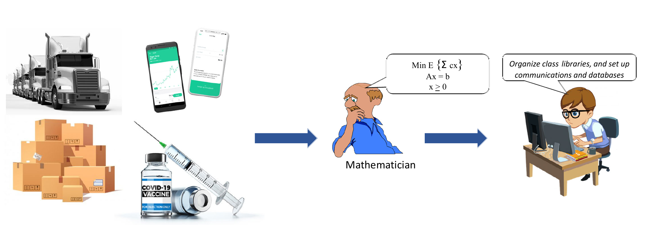
It is not necessary to understand equations $\eqref{eq:linearprogram1}$–$\eqref{eq:linearprogram3}$ (which requires basic familiarity with linear algebra), but thousands of students graduate each year from courses where they learn this notation, and also learn how to translate a wide range of physical problems into this notation. Then, there are software packages that translate problems in this format into a solution. Most important, this notational language is spoken around the world. The same statement can be made about statistical modeling/machine learning which today is a much larger community than the people who understand equations $\eqref{eq:linearprogram1}$–$\eqref{eq:linearprogram3}$.
We cannot make the same statement about sequential decision problems which is a problem class that is studied by at least 15 different communities using eight fundamentally different notational styles, often using mathematics that requires advanced training. In this book, we use a teach-by-example style to show how to model the incredibly rich class of problems that we call sequential decision problems. While we focus on relatively simpler problems, our framework can be used to model any sequential decision problem. In addition, the resulting model can be translated directly to software.
The analytical foundation of this book is contained in Reinforcement Learning and Stochastic Optimization: A unified framework for sequential decisions (RLSO) which is a graduate level text centered on methodology. From time to time we will refer to material in this book for readers who might be interested in greater depth, and we encourage technically inclined readers to use RLSO as a reference. However, it is not needed. This book is designed to provide the contextual background in the form of a series of examples that should enable readers to think clearly and precisely about sequential decision problems, even if they will never write a line of code.
This book is aimed at undergraduate or masters level students who have taken a course in probability and statistics (a knowledge of linear programming is not necessary, although we have an example which requires solving a linear program). All the chapters are built around specific examples, with the exception of chapter 1, which provides an overview of the entire modeling framework, and chapter 7, where we pause and use the first six chapters to illustrate some important principles.
The presentation should not require mathematics beyond what would be expected in a first course on probability and statistics. This said, the book is centered on showing how to describe sequential decision problems using notation that is precise enough that it can be the basis of computer software.
Python modules accompany most of the chapters; these modules were written around the modeling framework that runs throughout the book. At the same time, any software package that simulates a sequential decision problem, regardless of how it is being solved, can be translated directly into the modeling framework we use. For this reason, we encourage readers to look at any piece of notation as a variable in a computer program.
Getting started
Sequential decision problems can always be written as
\[decision,\ information, \ decision, \ information, \ decision, \ldots\]Each time we make a decision we incur a cost or receive a contribution or reward (there are many ways to measure performance). Decisions are made with a method that we are going to refer to as a policy. A major goal that is a central focus of this book is to design effective policies that work well over time, in the presence of the uncertainty of information that has not yet arrived.
Sequential decision problems are ubiquitous, arising in virtually every human process. Table 1.1 provides a sample list of fields, with examples of some of the decisions that might arise. Most of these fields probably have many different types of decisions, ranging in complexity from when to sell an asset or to adopt a new web design, to choosing the best drug, material, or facility to design, to managing complex supply chains or dispatching a fleet of trucks.
| Field | Questions |
|---|---|
| Business | What products should we sell, with what features? Which supplies should you use? What price should you charge? |
| Economics | What interest rate should the Federal Reserve charge given the state of the economy? What levels of market liquidity should be provided? |
| Finance | What stocks should a portfolio invest in? How should a trader hedge a contract for potential downside? |
| Internet | What ads should we display to maximize ad-clicks? Which movies attract the most attention? When/how should mass notices be sent? |
| Engineering | How to design devices from aerosol cans to electric vehicles, bridges to transportation systems, transistors to computers? |
| Public health | How should we run testing to estimate the progression of a disease? How should vaccines be allocated? Which population groups should be targeted? |
| Medical research | What molecular configuration will produce the drug which kills the most cancer cells? What set of steps are required to produce single-walled nanotubes? |
| Supply chain mgmt. | When should we place an order for inventory from China? Which supplier should be used? |
| Freight transportation | Which driver should move a load? What loads should a truckload carrier commit to move? Where should drivers be domiciled? |
| Information collection | Where should we send a drone to collect information on wildfires or invasive species? What drug should we test to combat a disease? |
| Multiagent systems | How should a large company in an oligopolistic market bid on contracts, anticipating the response of its competitors? |
| Algorithms | What stepsize rule should we use in a search algorithm? How do we determine the next point to evaluate an expensive function? |
Table 1.1. A sample of different fields and decisions that need to be made within each field.
Even more challenging than listing all the types of decisions is identifying the different sources of uncertainty that arise in many applications. Human behavior, markets, physical processes, transportation networks, energy systems and the broad array of uncertainties that arise in health hint at the diversity of different sources of uncertainty.
As this book is being written, humanity is struggling with the spread of variations of COVID-19. Dealing with this pandemic has been described as “mind-bogglingly complex,” [USA Today, Sept 8, 2020] but this is really a byproduct of a failure to think about the problem in a structured way. We are going to show the reader how to break down problems into a series of basic components that lead to practical solutions.
Our approach starts by identifying some core elements such as performance metrics, decisions, and sources of uncertainty, which then leads to the creation of a mathematical model of the problem. The next step is usually (but not always) to implement the model on the computer, but there are going to be many problems where the process of building a computer model is impractical for any of a number of reasons. For this reason, we are also going to consider problems where we have to test and evaluate ideas in the field. To improve performance, we need to first learn how to make good decisions over time (this is how we control the system). Then, we turn to the design of the system.
At this time, the academic community has not adopted a standard modeling process for sequential decision problems. This is in sharp contrast with the arena of static, deterministic optimization problems which have followed a strict framework since the 1950s (equations $\eqref{eq:linearprogram1}$–$\eqref{eq:linearprogram3}$ represent a sample of this framework). Our modeling process is based on the presentation in RLSO, which is a book aimed at a technical audience that is primarily interested in developing and implementing models on the computer.
By contrast, this book is aimed at a broader audience that is first and foremost interested in learning how to think about sequential decision problems. It uses a teach-by-example style that focuses on communicating the modeling process which we feel can be useful even without ultimately creating computer models. Central to our approach is the creation of a mathematical model that eliminates the ambiguity when describing problems in plain English. For readers who are interested in developing computer models, notation is the stepping stone to writing software. However, we are going to primarily use mathematical notation to create clarity when describing a problem, even if the reader never intends to write a line of code.
Our presentation proceeds as follows:
- Chapter 1 provides a light introduction to the universal modeling framework, illustrated using two inventory problems (a simple one, and one that is slightly more complex), followed by a brief discussion of modeling uncertainty. It then provides an introduction to the four classes of policies that cover every method for making decisions.
- Chapters 2–6 each describe a specific sequential decision problem to illustrate the modeling framework using a teach-by-example style. These applications were chosen to bring out each of the four classes of policies.
- Chapter 7 returns to the universal modeling framework in more detail. A much more careful discussion is given of the four classes of policies as well as different types of state variables, using the examples in chapters 2–6 to provide context.
- Chapters 8–14 provide additional examples, using more complex settings to illustrate more advanced modeling concepts, covering both uncertainty modeling (in particular the modeling of electricity prices in Chapter 8) and a richer set of policies.
The application chapters (2–6 and 8–14) all follow the same outline. They can be covered in any order, keeping in mind that the applications in chapters 2–6 are simpler and were chosen to illustrate each of the four classes of policies. Readers interested in specific modeling topics (such as state variables, modeling uncertainty, or seeing different examples of policies) may skim chapters, jumping directly to the topics that interest them.
Each chapter closes with a series of exercises divided into three categories:
- Review questions – These are simple questions that can be used to reinforce a basic understanding from reading the chapter.
- Problem solving questions – These introduce modeling challenges that require problem solving skills.
- Programming questions – Most chapters have programming exercises that draw on a set of Python modules. The original Python modules, written in Python 2, benefited from a major upgrade by Professor Dennis Djanka, a professor at Karlsruhe University in Germany. The new library can be downloaded from tinyurl.com/sdagithub. Some of these questions require making programming modifications to the Python code.
So, what is a decision?
There is a long history, dating back over 2,000 years to the days of Socrates, Aristotle and Plato, documenting the study of how people make decisions. Then there is a substantial literature, mostly since the 1950s (but with some important work before) on the mathematics of making optimal decisions, consisting of many thousands of papers and books. What this literature seems to overlook is the basic question:
What is a decision?
We start with the observation that a decision is a form of information that affects the behavior of some “system” that we are looking to control. Implicit in this system is one or more measures that quantify how well our system is performing. We then have to identify an agent that controls some aspect of our system.
Given this foundation, it helps to identify three classes of information:
- The state of knowledge – This is information that we have right now that is relevant to the performance of our system.
- Information that changes the state of knowledge that we control (this requires identifying a controlling agent for our system).
- Information arriving to our system that changes the state of knowledge that is beyond our control.
We refer to information in class 2 as decisions. This suggests a formal definition of a decision, drawing on Bridging Decision Problems, Volume I: Framing the Problem:
Definition (formal): A decision is an endogenously controllable information class.
An informal definition might be:
Definition (informal): A decision is information we control.
These definitions offer a starting point, but we do not learn very much from them. Much more interesting is to identify specific examples of decisions, which we do next.
Types of decisions
We have identified 10 types of decisions basic on the settings and the tools we might use to determine the best decisions. These are:
1) Physical and financial decisions – These decisions arise in the management of physical and financial resources, such as people, equipment, facilities, products, water, energy, as well as financial resources such as cash or investments. Decisions include buying, selling and modifying resources, where a modification might mean moving it from one location to another, repairing equipment, training a person, or combining ingredients to make a cake.
2) Complex/strategic decisions – These are decisions that may make multiple changes to a system (changing resources, parameters, beliefs), and which typically involve significant sources of uncertainty. These decisions are typically evaluated once, but the option of waiting and making the decision later may exist.
3) Information acquisition/observation decisions – These include decisions such as running experiments in the lab, field tests, or computer simulations. It might include performing market research, hiring an expert, or asking a large language model.
4) Information communication/sharing decisions – These come in two forms:
- a) Messaging – This reflects what we say in text, video and/or audio.
- b) Channels and timing – This covers the choice of how to send the information: text/emails, publication (print or online), social media, or advertising channels. It also requires choosing the timing and frequency.
5) Performance metrics and objectives – These represent the critical choice of quantifying what we are trying to achieve, such as maximizing revenues, minimizing costs, minimizing illness, or maximizing votes received.
6) Choosing functions – These may be methods to make decisions (policies), the formulation of optimization models, the choice of performance metrics, methods for forecasting or estimation, or the design of transition functions (such as how disease spreads).
7) Setting parameters – There are often a number of parameters that affect the performance of a system. These could be prices, the coefficients in a statistical model, the temperature used in a manufacturing process. They might be the weight placed on a performance metric, or performance targets.
8) Estimation or identification – We may need to identify a person, forecast demand, or name a disease.
9) Features and behaviors – How to design a product, what features a software package should have, what services should be provided to a customer, or a student’s major, which determines what skills they graduate with.
10) Deciding what to decide – While we generally do not use formal analysis for this final decision, it is important to recognize when we are making a decision, and whether we want to address it formally using data analysis and modeling.
Implicit in the identification of decisions is understanding how the decision affects the performance of the system. Moving physical resources (type 1) comes with a cost, while satisfying demands brings revenues. A decision may have an immediate impact on one or more performance metrics (as often occurs with managing resources), but often decisions have to be evaluated over time, and depend on information that is not known when the decision is made. For this reason, we are often evaluating how we are making decisions (that is, the method) as opposed to the decision itself.
Framing the problem
The first step when approaching a decision problem involves answering three questions:
- What are the performance metrics?
- What types of decisions are being made (and who makes them)?
- What are the uncertainties that affect performance?
Note that the answers to these questions are fundamental to any decision problem. In this book, these questions will seem fairly simple, because we answer them in the context of the models that we have already designed to solve a problem. In real applications, the lists of performance metrics, decisions, and uncertainties can be quite long.
As a hint of the richness that framing a problem can take on, we encourage the reader to look at the monograph Framing the Problem which is dedicated to just this topic. The monograph has entire chapters dedicated to each of these questions, which are illustrated using a dozen different applications.
The goal of the framing process is to identify what matters, starting with the performance metrics, where even a simple inventory problem can be described with over 20 performance metrics, 30 different types of decisions and over 30 types of uncertainties. The spreadsheet listing these can be found at tinyurl.com/PowellInventoryDecisions. This does not mean that we will actually build a model with all this complexity. For this reason, the book introduces a device called interaction matrices where a domain expert prioritizes the metrics, and then uses judgment to identify the decisions and uncertainties that have the largest impact on the most important metrics.
This book assumes we have already reduced a problem to a small number of metrics, decisions, and uncertainties, and uses these to focus the development of a mathematical model.
The modeling process
Modeling is an art, but it is art guided by a mathematical framework that ensures that we get a well-defined problem that we can put on the computer and solve. This can be viewed as building a bridge from a messy, poorly defined real-world problem to something with the clarity a computer can understand, even if your end goal is not to put it on the computer.
Historically, if a modeling effort involved trying to make decisions, people would turn to the well-known framework of deterministic optimization which often looks like the model given by equations $\eqref{eq:linearprogram1}$–$\eqref{eq:linearprogram3}$ which consists of decision variables $x$, an objective function $cx$, and the constraints given by $\eqref{eq:linearprogram2}$–$\eqref{eq:linearprogram3}$.
The problem with this classical modeling framework is what it leaves out:
- It assumes all the data (contained in the variables $A$, $b$ and $c$) characterizing the model is known perfectly.
- Most decisions occur repeatedly over time, and yet there is no recognition of this.
- There is no way to represent the flow of information to the system.
- As a byproduct, the optimal solution to this model cannot anticipate events that affect the performance of $x$ in the field.
- There is no way to represent risk, a major issue in many applications.
- It assumes a single decision-maker.
Mathematical models should, first and foremost, provide a path that tells us how to think about problems. The classical deterministic optimization models that follow the format of equations $\eqref{eq:linearprogram1}$–$\eqref{eq:linearprogram3}$ completely ignore anything related to the evolution of our problem over time.
This book is designed entirely around a modeling approach called the universal modeling framework. In a nutshell, it aspires to represent any aspect of a controllable system. Our default model will assume that the system evolves over time, as new information arrives.
In this section, we are going to provide a very compact version of the universal modeling framework. Then we are going to illustrate the framework, initially using a very simple inventory problem but then introducing some modest extensions. After presenting these examples, we are going to return to a more detailed presentation of the universal modeling framework.
A compact presentation of a dynamic model
We begin by observing that we can model any sequential decision problem using the sequence
\[(S_0,x_0,W_1,S_1,x_1,W_2, \ldots, S_t, x_t, W_{t+1}, \ldots, S_T),\]where:
- $S_t$ is the state variables that captures everything we need to:
- a) Make a decision at time $t$.
- b) Compute the performance metrics at time $t$.
- c) Any other information needed to compute (a) or (b) at any point in the future.
It is best to think of $S_t$ as the state of information or, more generally, the state of knowledge, at time $t$.
- $x_t$ represents decision variables which capture the elements that we control, such as whether to sell a house, the path through a network, the choice of drug for a treatment, the price at which to sell a product, or the choice of truck to move a load of freight.
-
$W_{t+1}$ is the information that arrives after we make the decision $x_t$, which might be the final selling price of a house, the travel times through a network, how a patient responds to a drug, the sales of a product at a price, and the loads of freight called in after we make initial assignments. We view the information in $W_{t+1}$ as coming from outside of our system, which means it is outside of our control. For this reason, we refer to it as exogenous information.
There are many settings where it is best to think of $W_{t+1}$ as a function $W_{t+1}(S_t,x_t)$ that depends on the current state $S_t$ and/or the decision $x_t$. We discuss this in more detail below. We are going to use $W_{t+1}$ as our default notation, but with the understanding that it may be influenced by the state $S_t$ or decision $x_t$.
The decision $x_t$ is determined by some method that we refer to as a policy, which we denote $X^\pi(S_t)$. The notation $\pi$ carries information about the structure of the function, which we represent by $f$ in a set of potential functions $\Fcal$, and any tunable parameters $\theta\in\Theta^f$, which is defined by the structure of the function. For example, an inventory policy might be to order $\theta^{order}$ units any time the inventory goes below $\theta^{min}$, which means the tunable parameters are $\theta = (\theta^{order}, \theta^{min})$. The structure of the function would be one example of a function $f$.
We assume we have a transition function that takes as input the state $S_t$, decision $x_t$, and the exogenous information $W_{t+1}$ and gives us the updated state $S_{t+1}$. Transition functions are a set of equations that update each element of the state variable $S_t$, which might have just one element, or tens of thousands (or much more).
We incur a contribution (or cost) $C(S_t,x_t)$ when we make the decision $x_t=X^\pi(S_t)$ given the information in state $S_t$. Our goal is to find the policy that maximizes some objective that depends on the contributions $C(S_t,x_t)$ where $x_t=X^\pi(S_t)$. For more complex settings, $C(S_t,x_t)$ can actually be a set of performance metrics, although we will need to combine them in a way to identify which decision $x_t$ to choose.
This is a very compact description of a sequential decision problem. We next describe a set of steps to follow in the modeling process.
The steps in the modeling process
It is possible to divide the entire modeling process into seven steps (for our purposes). Preceding these steps (labeled below as “Step 0”) is a brief summary of the technical complexity of the application to help guide readers.
Step 0. Chapter summary – We open each chapter with a summary of what the chapter is going to cover and, in some cases, how it relates to the material from other chapters. The summaries indicate what approaches are used to modeling uncertainty and the policies that are used.
Step 1. The narrative – This will be a plain English description of the problem. The narrative will not provide all the information needed to create a mathematical model; rather, it is a first step that should give the modeler the big picture without getting lost in notation.
Step 2. Framing the problem – This consists of answering three questions:
- What are the performance metrics?
- What types of decisions are being made (and in some cases, which agent is making them)?
- What are the sources of uncertainty that affect performance?
Step 3. Identifying the core elements of the problem, with special emphasis on three dimensions of any sequential decision problem. These elements are described without using mathematics:
- What metrics are we trying to impact? Individual fields (such as supply chain management, health, energy, finance) will each be characterized by a number of metrics that might be described using terms such as costs, revenues, profits, rewards, gains, losses, performance and risk.
- What decisions are being made? Identifying decisions is quite easy for many problems such as computer games, but if we address a complex problem such as responding to a public health process, reducing the carbon footprint, or managing a supply chain, then identifying all the decisions can be quite challenging.
- What are the different sources of uncertainty? What are we uncertain about before we start? What information arrives exogenously over time (that is, arrives after we make a decision)? Table 1.2 illustrates different sources of uncertainty for a model of the distribution of COVID vaccines (see RLSO, Chapter 10, for a presentation of 12 classes of uncertainty).
We refer to the process of answering these three questions as framing the problem.
| Type of uncertainty | Description |
|---|---|
| 1) Observational errors | Observing people with symptoms; errors classifying people with symptoms as having COVID |
| 2) Exogenous uncertainty | Reports of new cases, deaths; availability of ICUs; actual production of vaccines |
| 3) Prognostic uncertainty | Hospital admissions; future performance of vaccines; population response to vaccines |
| 4) Inferential uncertainty | Estimates of infection rates; estimates of effectiveness of vaccines |
| 5) Experimental uncertainty | Drug performance in a clinical trial; number being vaccinated |
| 6) Model uncertainty | Disease transmission rates; geographical spread of infections |
| 7) Transitional uncertainty | Additions/withdrawals to/from vaccine inventories |
| 8) Control uncertainty | Which population groups were vaccinated; vaccine allocations |
| 9) Implementation uncertainty | Failure to vaccinate |
| 10) Communication errors | Reporting errors from the field; failure to notify when to be vaccinated |
| 11) Goal uncertainty | Disagreements in who should be vaccinated |
| 12) Environmental uncertainty | If/when a vaccine will be approved; allocation of vaccines to different states, countries |
Table 1.2. Illustration of different types of uncertainty arising in the vaccination response to the COVID pandemic.
Step 4. The mathematical model – Here we build off the first three elements from Step 2, but now we have to create a mathematical model that consists of five dimensions that apply to every sequential decision problem:
- State variables $S_t$ – The state variable captures everything you need to know at time $t$ to make a decision at time $t$, compute costs and constraints, and if necessary, simulate your way to time $t+1$. State variables can include information about physical resources (inventories or the location of a vehicle which enter the problem through constraints), other information (such as costs or prices which enter the objective function), and beliefs about quantities and parameters we do not know perfectly (such as forecasts or estimates of how a patient would respond to a drug).
-
Decision variables $x_t$ – These describe how we are going to design or control our system. Decisions have to satisfy constraints that we write as $x_t \in \Xcal$ where $\Xcal$ could be a set of discrete choices, or a set of linear equations. Decisions will be determined by policies that are functions (or rules) that we designate by $X^\pi(S_t)$ that determine $x_t$ given what is in the state variable. Policies can be very simple (buy-low, sell-high) or quite complex.
The index $\pi$ carries information about the type of function that is used to make decisions, and any tunable parameters. Let $f\in\Fcal$ be the structure of the function, $\Fcal$ be the set of possible functions, and let $\theta\in\Theta^f$ be any tunable parameters for function $f$. Our policy would then be represented as $\pi = (f,\theta)$. We will often write the policy as $X^\pi(S_t\vert \theta)$ to indicate the dependence on tunable parameters.
We return to this in considerable detail later in this chapter, and throughout the book. Each of the examples given in the book has been chosen to help illustrate specific types of policies.
- Exogenous information $W_{t+1}$ – This is new information that arrives after we make decision $x_t$ (but before we decide $x_{t+1}$) such as how much we sell after setting a price, or the time to complete the path we chose. When we make a decision at time $t$, the information in $W_{t+1}$ is unknown, so we treat it as a random variable when we are choosing $x_t$.
- The transition function $S^M(S_t,x_t,W_{t+1})$ – These are the equations that describe how the state variables evolve over time. For many real problems, transition functions capture all the dynamics of the problem, and can be quite complex. In some cases, we do not even know the equations, and have to depend on just the state variables that we can observe. We write the evolution of the state variables $S_t$ using our transition function as
where $S^M(\cdot)$ is known as the state (or system) transition model (hence the $M$ in the superscript). The transition function describes how every element of the state variable changes given the decisions $x_t$ and exogenous information $W_{t+1}$. In complex problems, the transition function may require thousands of lines of code to implement.
-
The objective function – This captures the performance metrics we use to evaluate our performance, and provides the basis for searching over policies. We let $C(S_t,x_t)$ denote the contribution (if maximizing) or cost (if minimizing) of decision $x_t$ which may depend on the information in $S_t$. In some settings it is more natural to write the single-period contribution function as $C(S_t,x_t,W_{t+1})$, the contribution function evaluated at the end of time interval $(t,t+1)$, after $W_{t+1}$ has been observed. For example, we may place an order for $x_t$ that arrives right away to meet the uncertain demand contained in $W_{t+1}$.
Our objective is to find the best policy $X^\pi(S_t)$ to optimize some metric such as:
- Maximize the expected sum of contributions over some horizon.
- Maximize the expected performance of a final design that we learned over a number of experiments or observations.
- Minimize the risk associated with a final design.
Our most common way of writing the objective function is
where “$\E$” is called the expectation operator which means it is taking an average over anything random, which might include uncertain information in the initial state $S_0$, as well as the exogenous information process $W_1, \ldots, W_T$. It is standard to write the expectation operator, but we can never actually compute it. Later we show how to approximate it by running a series of simulations and taking an average, or by observing a process in the field.
Caution has to be used when interpreting the expectation operator “$\E$” in equation $\eqref{eq:baseobjectivefunction}$. What this operator literally means is to “take an average over anything that is uncertain.” The most obvious piece of uncertainty is the exogenous information process $W_1, W_2, \ldots, W_t, \ldots, W_T$.
The transition from the real problem (guided by the narrative) to the elements of the mathematical model is perhaps the most difficult step, as it often involves soliciting information from a non-technical source.
We note that we have presented the entire model without specifying how we make decisions, which is represented by the policy $X^\pi(S_t)$. We call this “model first, then solve” and it represents a major departure from the vast literature that deals with sequential decision problems. It is hard to communicate how important it is to approach sequential decision problems in this way.
Step 5. The uncertainty model – This is how we model the different types of uncertainty. There are two ways of introducing uncertainty into our model:
- Through the initial state $S_0$ which might specify a probability distribution for uncertain parameters such as how a patient might respond to a drug or how the market might respond to price.
- Through the exogenous information process $W_1, \ldots, W_T$.
We have three ways of modeling the exogenous information process:
- Create a mathematical model of $W_1, W_2, \ldots, W_T$.
- Use observations from history, such as past prices, sales, or weather events.
- Run the system in the field, observing $W_t$ as they happen.
Step 6. Designing policies – Policies are functions, so we have to search for the best function. (Yes, policies are functions to choose the best decision, but choosing the policy is also a decision!) We do this by identifying two core strategies for designing policies:
- Search over a family of functions to find the one that works best, on average, over time.
- Create a policy by estimating the immediate cost or contribution of a decision $x_t$, plus an approximation of future costs or contributions, and then finding the choice $x_t$ that optimizes the sum of current and future costs or contributions. Google Maps decides whether to turn left or right by optimizing over the time required to traverse the next link in the network plus the remaining time to get to the destination. An inventory decision might optimize over the cost of an order plus the estimated value of holding a certain amount of inventory moving forward.
We are going to be much more explicit about how to identify these policies. A later section describes four classes of policies that will include any method for making decisions (these are meta-classes).
Step 7. Evaluating policies – Finding the best policy means evaluating policies to determine which is best. There are two ways to evaluate a policy:
- Testing the policy in a computer simulator. This requires programming all the equations in the state transition model $S^M(S_t,x_t,W_{t+1})$ required to update the state variable $S_t$. It also means being able to generate samples of $W_{t+1}$, which is often the most subtle aspect of a simulator.
- Observing how the policy works in the field.
Simulators can be complex and difficult to build, and are still subject to modeling approximations. For this reason, the vast majority of practical problems encountered in practice tend to involve testing in the field, which is slow (it takes a day to simulate a day) and requires living with the results of the experiments.
The only way to become comfortable with a mathematical model is to see it illustrated using a familiar example. We start with a universal problem that we all encounter in everyday life: managing inventories.
Some inventory problems
We are going to illustrate our modeling framework using two variations of a classic inventory problem, which is widely used as an application for illustrating certain methods for solving sequential decision problems. We start with a simple inventory example that gets across the core elements of our modeling framework, but allows us to ignore many of the complexities that we will be exploring in the remainder of the book.
Then, we are going to transition to a slightly more complicated inventory problem that will allow us to illustrate some modeling principles. Throughout the book, we are also going to use the idea of starting with a basic version of a problem, and then introduce extensions that hint at the types of complications that can arise in real applications.
A simple inventory problem
One of the most familiar sequential decision problems that we all experience each time we visit a store is an inventory problem. We are going to use a simple version of this problem to illustrate the six steps of our modeling process that we introduced above:
Step 1: Narrative – A pizza restaurant has to decide how many pounds of sausage to order from its food distributor. The restaurant has to make the decision at the end of day $t$, communicate the order which then arrives the following morning to meet tomorrow’s orders. If there is sausage left over, it can be held to the following day. The cost of the sausage, and the price that it will be sold for the next day, is known in advance, but the demand is not.
Step 2: The core elements of the problem are:
- Metrics – We want to maximize profits given by the sales of sausage minus the cost of purchasing the sausage.
- Decisions – We have to decide how much to order at the end of one day, arriving at the beginning of the next.
- Sources of uncertainty – The only source of uncertainty in this simple model is the demand for sausage the next day.
Step 3: The mathematical model – This consists of five elements.
1) The state variable $S_t$ – We distinguish between the initial state variable $S_0$, and the dynamic state variable $S_t$ for $t > 0$. The initial state variable $S_0$ consists of fixed parameters and initial values of variables that change over time, giving us
\[S_0 = (R^{inv}_0, (p, c), (\Dbar, \sigmabar^D)).\]We have divided the initial state into three types of variables:
- Initial values of the resource state $R^{inv}_0$.
- Values of constant parameters $c$ and $p$.
- Our belief about the demands, given by a normal distribution with mean $\Dbar$ and standard deviation $\sigmabar^D$.
The dynamic state variable $S_t$ is our inventory which we are going to call $R^{inv}_t$. For now, this is the only element of the dynamic state variable, so
\[S_t = R^{inv}_t.\]Later we are going to introduce additional elements to our state variable.
2) The decision variable $x_t$ is how much we order at time $t$, which we assume (for now) arrives right away. We make our decisions with a policy $X^\pi(S_t)$ which we design later.
3) The exogenous information is the random demand for our product which we are going to denote $\Dhat_{t+1}$, so $W_{t+1} = \Dhat_{t+1}$.
4) Our transition function captures how the inventory $R_t$ evolves over time, which is given by
\[\begin{align} R^{inv}_{t+1} = \max\{0, R^{inv}_t+x_t-\Dhat_{t+1}\}. \label{eq:inventoryexampleequation} \end{align}\]5) Our objective function. For our inventory problem, it is most natural to compute the contribution including the purchase cost of product $x_t$ and the revenue from satisfying the demand $\Dhat_{t+1}$, which means that our single-period contribution function would be written
\[C(S_t,x_t,\Dhat_{t+1}) = -cx_t + p \min\{R^{inv}_t+x_t, \Dhat_{t+1}\},\]where $x_t = X^\pi(S_t)$. Given a sequence of demands $\Dhat_1, \ldots, \Dhat_T$, the value of a policy $\Fhat^\pi$ would be
\[\Fhat^\pi(S_0) = \sum_{t=0}^T C(S_t,X^\pi(S_t),\Dhat_{t+1}).\]Our profits $\Fhat^\pi(S_0)$ are random because it depends on a particular sequence of random demands $\Dhat_1, \ldots, \Dhat_T$. Finally we average over these random demands by taking the expectation:
\[\begin{align} F^\pi(S_0) = \E \left\{\sum_{t=0}^T C(S_t,X^\pi(S_t),\Dhat_{t+1})\vert S_0\right\}. \label{eq:inventoryobjective} \end{align}\]Here, the conditioning on the initial state $S_0$ can be read as saying “take the expectation given what we know initially.” Conditioning on $S_0$ is implicit any time we take an expectation, and as a result many authors leave it out. However, we are going to include the conditioning on $S_0$ to make it clear that if our initial inputs (including beliefs) change, then this may have an effect on how a policy performs.
Step 4. The uncertainty model – The simplest approach to modeling uncertainty is to just use historical data. The problem we might encounter is that if we run out of sausage, we might not observe the full demand for sausage that day. If we are able to capture this lost demand, then this is a reasonable approach.
An alternative is to build a mathematical model. We might assume that our demand is normally distributed with some mean $\Dbar$ and standard deviation $\sigmabar^D$. If we assume that both of these are known, we can write our demand as
\[\Dhat_{t+1} \sim N(\Dbar,(\sigmabar^D)^2),\]and take advantage of packages that can sample from the normal distribution (for example, in Excel this is called Norm.inv$(Rand(),\Dbar,\sigmabar)$ to generate a random observation with mean $\Dbar$ and standard deviation $\sigmabar$.
Using this model, we can create a set of demands $(\Dhat_1, \Dhat_2, \ldots, \Dhat_T)$. Then, we can repeat this $N$ times to create $N$ sequences of $T$ demands, giving us the sequence $(\Dhat^n_1, \Dhat^n_2, \ldots, \Dhat^n_T)$ for $n=1, \ldots, N$ that we need to estimate the value of the policy (we use this below in Step 6).
Step 5. Designing policies – Next we have to design a method for determining our orders. A commonly used strategy for inventory problems is known as an “order-up-to” policy that looks like
\[\begin{align} X^\pi(S_t\vert \theta) = \begin{cases} \theta^{max} - R_t & \text{if } R_t < \theta^{min}, \\ 0 & \text{otherwise,}\end{cases} \label{eq:introorderupto} \end{align}\]where $\theta = (\theta^{min},\theta^{max})$ is a set of parameters that need to be tuned. It is called “order-up-to” since we place an order to bring the inventory “up to” the upper limit $\theta^{max}$.
Step 6. Evaluating policies – There are a variety of strategies we might use. In practice, we cannot compute the expectation in the objective function in equation $\eqref{eq:inventoryobjective}$, so we take a series of samples of demands. Let $\Dhat^n_1, \ldots, \Dhat^n_T$ be one sample of demands over $t=1, \ldots, T$, and assume we can generate $N$ of these. Now we can estimate our expected profits from policy $X^\pi(S_t)$ by averaging over the samples for $n=1, \ldots, N$, which is computed using
\[\Fbar^\pi(\theta\vert S_0) = \frac{1}{N} \sum_{n=1}^N \sum_{t=0}^T C(S_t,X^\pi(S_t\vert \theta),\Dhat^n_{t+1}).\]In plain English, we are simulating the policy $X^\pi(S_t\vert \theta)$ $N$ times using the simulated (or observed from history) samples of demands $\Dhat^n_1, \ldots, \Dhat^n_T$, and then averaging the performance to get $\Fbar^\pi(\theta\vert S_0)$. We then face the problem of finding the best value of $\theta$. A simple strategy would be to generate $K$ possible values $\theta_1, \ldots, \theta_K$, simulating each one to find $\Fbar^\pi(\theta_k\vert S_0)$ for each $k$, and then pick the value of $\theta_k$ that works the best. This is not an optimal strategy, but it provides a simple, practical starting point.
A slightly more complicated problem
The simple inventory problem above is a classic setting for demonstrating a particular method for solving sequential decision problems known as dynamic programming, which depends on having a simple state variable that is a) discrete and b) does not have too many possible values. In our slightly more complicated inventory problem, we are going to illustrate three different flavors of state variables which would represent a serious complication for one popular method for solving sequential decision problems, but has no effect on the policy that we have chosen.
Step 1: Narrative – We again have our pizza restaurant that has to order sausage, but we are going to allow the price we pay for sausage to vary from day to day, where we assume the price on one day is independent of the price on the previous day. Then, we are also going to assume that while the demand for sausage tomorrow is random, we are going to be given a forecast of tomorrow’s demand that, while not perfect, is better than not having a forecast. Otherwise, everything about our more complicated problem is the same as it was before.
Step 2: Core elements – These are:
- Metrics – We want to maximize profits given by the sales of sausage minus the cost of purchasing the sausage, where the cost varies from day to day.
- Decisions – As with our simpler inventory problem, we have to decide how much to order at the end of one day, arriving at the beginning of the next.
- Sources of uncertainty – There are now three sources of uncertainty: the difference between the actual demand and the forecast, the evolution of the forecasts from one day to the next, and the price we pay for the sausage.
Step 3: Mathematical model – We still have the same five elements, but now the problem is a bit richer:
1) To construct the state variable, we need to list the information (specifically, information that evolves over time) that is needed in three different parts of the model: (1) the objective function, (2) the policy for making decisions (which includes the constraints), and (3) the transition function. Of course, we have not yet introduced any of these functions, so you have to read forward, and verify that our state variable contains all the information needed to compute each of these functions. Think of this as a dictionary of the information we will need.
We start with the initial state $S_0$ which consists of constant parameters, and initial values of quantities and parameters that change over time. These are:
- Initial inventory – We start with an initial inventory $R_0$.
- Initial purchase cost – $c_0$.
- Price – We assume that we sell our sausage at a fixed price $p$.
- Initial forecast – We assume that our first forecast $f^D_{0,1}$ is given, where $f^D_{0,1}$ is the forecast known at time 0 for the demand at time 1.
- Initial estimate of the standard deviation of the demand – $\sigmabar^D_0$.
- Initial estimate of the standard deviation of the forecast – $\sigmabar^f_0$.
This means our initial state variable is
\[S_0 = (R_0,c_0, p, f^D_{0,1}, \sigmabar^D_0, \sigmabar^f_0).\]We then have the information that evolves over time which makes up our dynamic state variable $S_t$:
- Current inventory $R^{inv}_t$ – The inventory for the beginning of time interval $(t,t+1)$.
- Purchase cost $c_t$ – This is the cost of sausage purchased at time $t$ which is given to us at time $t$.
- Demand forecast $f^D_{t,t+1}$ – This is the forecast of $\Dhat_{t+1}$ given what we know at time $t$.
- Current estimate of the standard deviation of the demand – $\sigmabar^D_t$.
- Current estimate of the standard deviation of the forecast – $\sigmabar^f_t$.
Our dynamic state variable is then given by
\[S_t = (R^{inv}_t, c_t, f^D_{t,t+1}, \sigmabar^D_t, \sigmabar^f_t).\]2) The decision variable $x_t$ is how much we order at time $t$, which we assume (for now) arrives right away. We make our decisions with a policy $X^\pi(S_t)$ which we design later.
3) The exogenous information now consists of:
- Purchase costs $\chat_{t+1}$ – This is the purchase cost of sausage on day $t+1$ which is specified exogenously.
- Forecasts – Each time period we are given a new forecast. Let $\varepsilon^f_{t+1}$ be the change in the forecast between time $t$ and $t+1$.
- Demands – Finally, we assume that the actual demand is a random deviation from the forecast, which we could write
Our complete set of exogenous information variables can now be written
\[W_{t+1} = \big(\chat_{t+1}, \varepsilon^f_{t+1}, \varepsilon^D_{t+1}\big).\]4) Transition function – This specifies how each of the (dynamic) state variables $S_t$ evolve over time. We update our inventory using:
\[\begin{align} R^{inv}_{t+1} &= \max\{0, R^{inv}_t + x_t - \Dhat_{t+1}\}. \label{eq:introcomplexinventorytransition1} \end{align}\]The demand is the forecasted demand plus the deviation $\varepsilon^D_{t+1}$ from the forecast, giving us the equation:
\[\begin{align} \Dhat_{t+1} &= f^D_{t,t+1} + \varepsilon^D_{t+1}. \label{eq:introcomplexinventorytransition2} \end{align}\]We assume that our forecast is updated using
\[\begin{align} f^D_{t+1,t+2} &= f^D_{t,t+1} + \varepsilon^f_{t+1}. \label{eq:introcomplexinventorytransition3} \end{align}\]Next, we are going to adaptively estimate the variance in the demand and the demand forecast:
\[\begin{align} (\sigmabar^D_{t+1})^2 &= (1-\alpha)(\sigmabar^D_t)^2 + \alpha (f^D_{t,t+1} - \Dhat_{t+1})^2, \label{eq:introcomplexinventorytransition4}\\ (\sigmabar^f_{t+1})^2 &= (1-\alpha)(\sigmabar^f_t)^2 + \alpha (f^D_{t,t+1} - f^D_{t+1,t+2})^2, \label{eq:introcomplexinventorytransition5} \end{align}\]where $0 < \alpha < 1$ is a smoothing factor.
Finally, we update the cost $c_{t+1}$ with the “observed cost” $\chat_{t+1}$ which we write simply as
\[\begin{align} c_{t+1} = \chat_{t+1}.\label{eq:introcomplexinventorytransition6} \end{align}\]Equation $\eqref{eq:introcomplexinventorytransition6}$ is an example of a state variable that we observe rather than compute, as we did with the inventory $R^{inv}_t$ in $\eqref{eq:introcomplexinventorytransition1}$. Equation $\eqref{eq:introcomplexinventorytransition1}$ is sometimes referred to as “model based,” since it reflects the physics of how inventories are updated, while equation $\eqref{eq:introcomplexinventorytransition6}$ is called “model free,” since we do not make any attempt at modeling the underlying process that produces the change in costs.
Our transition function $S_{t+1} = S^M(S_t,x_t,W_{t+1})$ consists of the equations $\eqref{eq:introcomplexinventorytransition1}$–$\eqref{eq:introcomplexinventorytransition6}$.
5) Finally, our single period contribution function would now be written
\[C(S_t,x_t,\Dhat_{t+1}) = -c_tx_t + p \min\{R_t+x_t, \Dhat_{t+1}\},\]where the only difference with the simpler inventory problem is that the cost $c$ is now time-dependent $c_t$. We break from our convention of writing the contribution as $C(S_t,x_t)$ and allow it to include revenues from the demands $\Dhat_{t+1}$.
We now state our objective function formally as
\[\begin{align} \max_{\pi=(f,\theta)} \E \left\{\sum_{t=0}^T C(S_t,X^\pi(S_t\vert \theta),\Dhat_{t+1})\vert S_0\right\}. \label{eq:introcomplexinventoryobjective} \end{align}\]The optimization $\max_\pi$ means that we are searching over all possible policies represented by $(f,\theta)$, which literally means searching over all the different functions we might use to make a decision. The examples in this book are going to demonstrate how we are going to search over functions.
Recall that above we stated that the index $\pi$ carries information about the type of function $f\in\Fcal$, and any tunable parameters $\theta\in\Theta^f$. In practice, the search over the types of functions $f\in\Fcal$ tends to be ad hoc (a knowledgeable analyst chooses functions that make sense for a problem), whereas a computer algorithm performs the search for the best value of $\theta\in\Theta^f$.
Step 4. The uncertainty model – We are going to assume that the exogenous changes $\varepsilon^D_{t+1}$ and $\varepsilon^f_{t+1}$ are described by normal distributions with mean 0 and variances $(\sigmabar^D_t)^2$ and $(\sigmabar^f_t)^2$, which we express by writing
\[\varepsilon^D_t \sim N(0, (\sigmabar^D_t)^2), \quad \varepsilon^f_t \sim N(0, (\sigmabar^f_t)^2).\]Uncertainty models can become quite complex, but this will serve as an illustration.
Step 5. Designing policies – Next we have to design a method for determining our orders. Instead of the order-up-to policy of our simpler model, we are going to suggest the idea of ordering enough to meet the expected demand for tomorrow, with an adjustment. We could write this as
\[\begin{align} X^\pi(S_t\vert \theta) = \max\{0,f^D_{t,t+1}-R_t\} + \theta. \label{eq:adjustedforecastpolicy} \end{align}\]If we had a perfect forecast, then all we have to order would be $f^D_{t,t+1}$ (our forecast of $\Dhat_{t+1}$) minus the on-hand inventory. However, because of uncertainty we are going to add an adjustment $\theta$ so that we have some buffer to avoid stockouts.
Step 6. Evaluating policies – This time we have to generate samples of all the random variables in the sequence $W_1, W_2, \ldots, W_T$. Again we might generate $N$ samples of the entire sequence so we can estimate the performance of a policy using
\[\Fbar^\pi(\theta) = \frac{1}{N} \sum_{n=1}^N \sum_{t=0}^T C(S_t,X^\pi(S_t\vert \theta),\Dhat^n_{t+1}).\]We again face the problem of finding the best value of $\theta$, but we return to that challenge later.
The universal modeling framework
We are now ready to describe in more detail the elements of the universal modeling framework (UMF). We note that the UMF can model any sequential decision problem. This fairly broad claim will become apparent as the elements unfold, since we are just applying notation to the general statement of a sequential decision problem.
The five elements of the UMF
The UMF consists of the following elements:
- The state variables $S_t$.
- The decision variables $x_t$.
- The exogenous information process $W_t$.
- The state transition model $S^M(S_t,x_t,W_{t+1})$.
- The objective function.
We describe these in more detail as follows:
State variables – The state $S_t$ of the system at time $t$ has all the information that is necessary and sufficient to model our system from time $t$ onward. More specifically, this information consists of:
- a) The information needed to make a decision at time $t$.
- b) The information needed to compute the performance metrics at time $t$.
- c) Any information needed now to compute (a) and (b) in the future.
There are three types of information in $S_t$:
- The physical state, $R_t$, captures physical quantities such as inventories, people, available machines, facilities, water, drugs, energy and money (in its various forms). $R_t$ will also include customer requests for products or services. In many applications $R_t$ describes the resource that is being managed, and a fairly common error is to equate “state” with “physical state.”
- The information state, $I_t$, which contains the functions being used (when there is a choice) and any tunable parameters. $I_t$ might specify how we are forecasting demands, and the parameters used to fit the forecast, in addition to any other parameters that control the evolution of the system.
- The belief state, $B_t$, which contains estimates or beliefs about quantities and parameters that are not known perfectly. Thus, $B_t$ could capture the estimated mean and variance of a normal distribution (as with our demand forecast above). Alternatively, it could be a vector of probabilities that evolve over time.
The physical state $R_t$ might be the amount of money in a cash account, while $I_t$ might be the current state of the stock and bond markets. If we are traveling over a dynamic network, $R_t$ might be our location on the network, while $I_t$ could be what we know about the travel times over each link. If we plan a path and then wish to penalize deviations from the plan, then the plan would be included in the state variable through $I_t$.
State variables typically are not obvious. They emerge during the modeling process, rather than something you can just immediately write out. Just because we write it first does not mean that you will always be able to list all the elements of the state variable right away. But in the end, this is where you store all the information you need to model your system from time $t$ onward.
Decision variables – Different communities use different notations for decision, such as $a_t$ for a (typically discrete) action or $u_t$ for a (typically continuous) control in engineering. We use $x_t$ as our default since it is widely used by the math programming community.
Decision variables come in different flavors:
- Binary (e.g. for modeling whether to sell an asset or not, or for A/B testing of different web designs).
- Discrete (e.g. choice of drug, which product to advertise).
- Continuous scalar (prices, temperatures, concentrations).
- Vectors (discrete or continuous such as allocations of blood supplies among hospitals).
- Categorical (e.g. what features to highlight in a product advertisement).
We note that there are classes of algorithms determined by the nature of the decision variable.
We assume that decisions are made with a policy, which we might denote $X^\pi(S_t)$ if we use $x_t$ as our decision. We assume that a decision $x_t = X^\pi(S_t)$ is feasible at time $t$, which means $x_t \in \Xcal_t$ for some set (or region) $\Xcal_t$, which may depend on $S_t$.
We let “$\pi$” carry the information about the type of function $f\in\Fcal$ (for example, a linear model with specific explanatory variables), and any tunable parameters $\theta \in \Theta^f$.
Exogenous information – We let $W_{t+1}$ be any new information that first becomes known at time $t+1$ (that is, between $t$ and $t+1$), where the source of the information is from outside of our system (which is why it is “exogenous”). When modeling specific variables, we use “hats” to indicate exogenous information. Thus, $\Dhat_{t+1}$ could be the demand that arises between $t$ and $t+1$, or we could let $\phat_{t+1}$ be the change in the price between $t$ and $t+1$.
The exogenous information process may be stationary or nonstationary, purely exogenous or state (and possibly action) dependent (if we decide to sell a lot of stock, it could push prices down).
We let $\omega$ represent a sample path $W_1, \ldots, W_T$, which represents a sequence of outcomes of each $W_t$. Often, we will create a set $\Omega$ of discrete samples, where each sample represents a particular sequence of the outcomes of our $W_t$ process which we could write as $W_1(\omega), \ldots, W_T(\omega)$. If we have 20 sample paths, we can think of $\omega$ as consisting of a number between 1 and 20, which allows us to look up the sample path.
Transition function – We denote the transition function by
\[\begin{align} S_{t+1} = S^M(S_t,x_t,W_{t+1}), \label{eq:transition} \end{align}\]where $S^M(\cdot)$ is also known by names such as state transition model, system model, plant model, plant equation, state equation, and transfer function.
Equation $\eqref{eq:transition}$ is the classical form of a transition function which gives the equations from the state $S_t$ to the state $S_{t+1}$. Equation $\eqref{eq:inventoryexampleequation}$ was the only transition equation for our simple inventory example, while equations $\eqref{eq:introcomplexinventorytransition1}$–$\eqref{eq:introcomplexinventorytransition6}$ made up the transition function for our more complicated example.
The transition function might capture any of the following types of updates:
- Changes in physical resources such as adding inventory, moving people, or modifying equipment.
- Updates to information such as changes in prices and weather.
- Updates to our beliefs about uncertain quantities or parameters.
The transition function may be a known set of equations, or unknown, such as when we describe human behavior or the evolution of CO2 in the atmosphere. When the equations are unknown the problem is often described as “model free” or “data driven” which means we can only observe changes in a variable, rather than using a physical model. Equation $\eqref{eq:introcomplexinventorytransition6}$, where we “observe” the cost $c_{t+1} = \chat_{t+1}$, with no idea how we evolved from $c_t$, is an example of a model free transition.
Transition functions may be linear, continuous nonlinear or step functions. When the state $S_t$ includes a belief state $B_t$, then the transition function has to include the updating equations (we illustrate this later in the book).
Given a policy $X^\pi(S_t)$, an exogenous process $W_{t+1}$ and a transition function, we can write our sequence of states, decisions, and information as
\[(S_0, x_0, W_1, S_1, x_1, W_2, \ldots, x_{T-1}, W_T, S_T).\]Objective functions – There are a number of ways to write objective functions. One of the most common, which we will use as a default, maximizes total expected contributions over some horizon $t=0, \ldots, T$
\[\begin{align} \max_{\pi=(f,\theta)} F^\pi(S_0) = \E \left\{\sum_{t=0}^T C_t(S_t,X^\pi_t(S_t\vert \theta))\vert S_0\right\}, \label{eq:objectivecumulativereward} \end{align}\]where
\[\begin{align} S_{t+1} = S^M(S_t,X^\pi_t(S_t),W_{t+1}). \label{eq:basetransition} \end{align}\]The model is fully specified when we also have a model of the initial state $S_0$, and a model of the exogenous process $W_1, W_2, \ldots$. We write all the exogenous information as
\[\begin{align} (S_0, W_1, W_2, \ldots, W_T). \label{eq:basestochasticmodel} \end{align}\]Equations $\eqref{eq:objectivecumulativereward}$, $\eqref{eq:basetransition}$ and $\eqref{eq:basestochasticmodel}$ constitute a model of a sequential decision problem.
Moving forward, for compactness we are going to use $\max_\pi$ to represent a search over the types of functions $f\in\Fcal$ and tunable parameters $\theta\in\Theta^f$.
Equation $\eqref{eq:objectivecumulativereward}$ uses an expectation $\E$ which means to take an average over all the possible outcomes of $W_1, \ldots, W_T$. This is virtually never possible to do computationally. Instead, let $\omega$ represent a single outcome of the sequence $W_1, \ldots, W_T$ which we might write $W_1(\omega), \ldots, W_T(\omega)$. Assume that we can create $N$ possible outcomes of this sequence, and let $\omega^n$ represent how we index the $n^{th}$ sequence.
If we are following a sample path $\omega$, we would then rewrite our transition function in $\eqref{eq:basetransition}$ using
\[\begin{align} S_{t+1}(\omega) = S^M(S_t(\omega),X^\pi_t(S_t(\omega)),W_{t+1}(\omega)). \label{eq:basetransition2} \end{align}\]We index every variable in equation $\eqref{eq:basetransition2}$ by $\omega$ to indicate that we are following a single sample path of values of $W_t$.
We can now replace our expectation-based objective with an average which we can write
\[\begin{align} \max_\pi \Fbar^\pi(S_0) = \frac{1}{N}\sum_{n=1}^N \sum_{t=0}^T C_t(S_t(\omega^n),X^\pi_t(S_t(\omega^n))). \label{eq:objectivecumulativerewardaverage} \end{align}\]Often, we are just working with a single sample path, possibly from history. In this case, we are approximating the performance of the policy using this single sample path, which we can write as
\[\begin{align} \max_\pi \Fhat^\pi(\omega\vert S_0) = \sum_{t=0}^T C_t(S_t(\omega),X^\pi_t(S_t(\omega))). \label{eq:objectivecumulativerewardsample} \end{align}\]Any time we write an objective using an expectation as in $\eqref{eq:objectivecumulativereward}$, remember that what we would really do is to use an average as we do in $\eqref{eq:objectivecumulativerewardaverage}$ or a sample as in $\eqref{eq:objectivecumulativerewardsample}$.
The expectation may also need to reflect uncertainty in the initial state $S_0$, which might capture beliefs about uncertain forecasts, or uncertain estimates about the state of disease in a patient. In this case, the sample path $\omega$ needs to include samples from these initial distributions.
There will be some settings where it makes more sense to use a counter $n$ rather than time. In this case, we let $S^n$ be the state after $n$ observations (these may be experiments, customer arrivals, iterations of an algorithm). We will use time $t$ as our default index.
The initial state variables $S_0$
We need to distinguish between the initial state $S_0$ and subsequent states $S_t$ for $t > 0$:
- $S_0$ – The initial state $S_0$ captures i) deterministic parameters that never change, ii) initial values of quantities or parameters that do change (possibly due to decisions), and iii) beliefs about quantities or parameters that we do not know perfectly (this might be the parameters of a probability distribution) such as how we respond to a vaccine or how the market will respond to price. The beliefs may remain static, or we may update them as we learn from observations.
- $S_t$ – This is all the information we need at time $t$ from history to model the system from time $t$ onward. $S_t$ for $t > 0$ only includes variables that are changing over time, which means that at time $t$ we may also be using static information contained in $S_0$.
We write the explicit dependence of the performance of the policy on the initial state $S_0$, whether we use $F^\pi(S_0)$, $\Fbar^\pi(S_0)$ or $\Fhat^\pi(\omega\vert S_0)$. While this should be obvious, it is often overlooked. The initial state includes elements such as:
- Initial values of the quantities of physical or financial resources $R_0$ – This might be starting inventories, the initial location of a vehicle, the available machines, and the initial set of facilities. It also includes any static values, such as a transportation network, the size of a warehouse (which does not change), and the number of trucks in a fleet.
- Initial values of parameters, along with any functions used to model the problem $I_0$ – This could be an initial price, the level of medication in a patient, along with the choice of functions for performing forecasting or modeling the evolution of disease in a population.
- Initial beliefs or estimates of any quantity or parameter $B_0$ – This could be a demand forecast, the estimate of how markets respond to prices, how a presidential candidate is polling, or beliefs in the performance of a manufacturing process.
We note it helps to separate initial values that never change, from those that evolve over time, either directly as a result of decisions or from exogenous information. Values that never change are stored in $S_0$, but are not represented in $S_t$ for $t > 0$. The reason for this is the desire to keep $S_t$ as compact as possible.
Assume our policy $X^\pi(S_t\vert \theta)$ has tunable parameters. For example, we might be managing an inventory system where we use the familiar “order-up-to” policy (known in the inventory literature as an $(s,S)$ policy) given by
\[X^\pi(S_t\vert \theta) = \begin{cases} \theta^{max} - R_t & R_t < \theta^{min},\\ 0 & \text{otherwise.}\end{cases}\]where $\theta = (\theta^{min},\theta^{max})$. For simplicity we might assume when we place an order it arrives right away (a standard textbook assumption that is never true in practice) which allows us to write the evolution of our physical state $R_t$ (the amount in inventory just before we place our instantaneous order) using
\[R_{t+1} = \max\{0,R_t + x_t - \Dhat_{t+1}\}\]where $x_t = X^\pi(S_t\vert \theta)$ and $\Dhat_{t+1}$ is the demand for our product over the interval $(t,t+1)$ (this is our exogenous information $W_{t+1}$). Finally let $C(S_t,x_t,W_{t+1})$ be our net profit over the interval $(t,t+1)$ (which is not important right now).
Now imagine that we have a historical demand process $W_1, W_2, \ldots, W_t, \ldots, W_T$ that allows us to run a simulation of our system. Let $\omega$ represent this historical sequence of demands (or any exogenous information). We would write the problem of finding the best set of ordering parameters $\theta$ using
\[\begin{align} \max_\theta \Fhat^\pi(\omega,\theta\vert S_0) = \sum_{t=0}^T C_t(S_t(\omega),X^\pi_t(S_t(\omega))), \label{eq:optimizingtheta} \end{align}\]where the state variable evolves according to
\[S_{t+1}(\omega) = S^M(S_t(\omega), X^\pi_t(S_t(\omega)), W_{t+1}(\omega)).\]Let $\theta^\ast $ be the value of $\theta$ that we found by optimizing $\eqref{eq:optimizingtheta}$. The proper way to write this optimal value is as a function $\theta^\ast (S_0)$ that depends on the information in $S_0$ (it also depends on the sample path $\omega$). This helps to communicate the reality that if we change the input data to our problem, represented by $S_0$, then this may have an impact on the best values of our policy parameters $\theta$. In fact, we might even have to change our choice of policy!
Variations
There are two important variations of our basic mathematical model:
-
From time $t$ to iteration $n$ – There are problem settings where it is more natural to use a counter $n$ than time $t$. We do more than just change $t$ to $n$ since we view variables that change with iterations differently from an evolution over time. Specifically, we put the index $n$ in the superscript, such as $S^n$, $x^n$ and $W^{n+1}$.
One reason for this is that we view a set of variables over time $x_1, x_2, \ldots, x_t, \ldots, x_T$ as a vector $x=(x_1, x_2, \ldots, x_t, \ldots, x_T)$, which is useful when modeling deterministic problems (we might optimize over the entire vector $x$ at once). By contrast, we view $x^n$ as a function that is evolving over time.
More practically, putting $n$ in the superscript allows us to write iterative simulations. So, we would write the information process over time for iteration $n$ using
If we are iteratively searching for the best policy, we might write our policy for iteration $n$ using $X^{\pi,n}(S_t)$, which then produces
\[S^n_0, x^n_0, W^n_1, \ldots, S^n_t, x^n_t, W^N_{t+1}, \ldots, S^N_T,\]where $x^n_t = X^{\pi,n}(S^n_t\vert \theta)$.
-
Optimizing final reward – A common setting is where we are performing stochastic search, as would happen when looking for the best policy. Each iteration for evaluating the algorithm might require a simulation over time, although this is not always the case.
Now let’s assume that our decision variable is the parameter $\theta$, and that we have an algorithm $\Theta^\pi(S^{\theta,n})$ that works just like a policy $X^\pi(S_t\vert \theta)$, but where $S^{\theta,n}$ captures the “state” of the algorithm at the $n$th iteration.
Search algorithms are all sequential decision problems, but unlike most sequential decision problems over time, we want to run $N$ iterations, and we only care about our solution at the end. Let $\theta^{\pi,N}$ be the value of $\theta^n$ after $N$ iterations, while following “algorithm” (policy) $\pi$.
The value $\theta^{\pi,N}$ depends on the specific sequence of our information process $W^1, \ldots, W^t, \ldots, W^N$, but we then have to evaluate it using a new set of samples that we are going to call $\What$.
We evaluate the performance of our algorithm using a final reward objective, which we write as
Stated simply, we evaluate our learning policy for $\theta$, which we denoted $\Theta^\pi(S^{\theta,N})$ by simulating through $N$ iterations using observations of $W^n$ (which may be an entire simulation over time $t$). When we obtain our final estimate of the parameter $\theta$, which we call $\theta^{\pi,N}$, we evaluate the performance of this value using a separate simulation where we fix $\theta = \theta^{\pi,N}$ and then create a new set of random observations that we call $\What^m$ for $m=1, \ldots, M$.
Modeling uncertainty
For many complex problems (supply chains, energy systems, and public health are just a few), identifying and modeling the different forms of uncertainty can be a rich and complex exercise. We are going to hint at the issues that arise, but we are not going to attempt a thorough discussion of this dimension.
Uncertainty is communicated to our model through two mechanisms: the initial state $S_0$, which is where we would model the parameters of probability distributions describing quantities and parameters that we do not know perfectly, and the exogenous information process $W_1, \ldots, W_T$.
Uncertainty in the initial state
The initial state variable may contain deterministic parameters or initial values of dynamically varying quantities and parameters. If this is all that is in the initial state, then it is not capturing any form of uncertainty.
There are many problems where we do not know some quantities or parameters, but can represent what we do know through the parameters of a probability distribution. Some examples are:
- The response of a patient to a new medication.
- How a market will respond to a change in price.
- How many salable heads of lettuce we have in inventory (an uncertain number may have wilted and are no longer salable).
- The time at which a box of inventory previously ordered from China will arrive.
- The amount of deposits to a mutual fund vary randomly around a mean $\lambda$, but we do not know what $\lambda$ is.
These are a number of ways that we can initialize a model with uncertainty in some of the inputs.
An initial probabilistic belief may come from subjective judgment, or from previous observations or experiments.
The exogenous information process
The second way uncertainty enters our model is through the exogenous information process. The variable $W_t$ contains information that is not known until time period $t$. This means we have to make a decision $x_t$ at time $t$ before we know the outcome of $W_{t+1}$.
Below is a list of examples of $W_{t+1}$ that are revealed after a decision $x_t$ is made:
- We choose a path, and then observe the travel time on the path.
- We choose a drug, and then observe how the patient responds.
- We choose a catalyst, and then observe the strength of the material that it produces.
- We choose a product to advertise in an online market, and then observe the sales.
- We select a web interface design, and then observe the number of clicks that it can generate.
- We allocate funds into an investment, and then observe the change in the price of the investment.
In each case, the information we observe after we make the decision affects the performance of the decision (and which decision would have been best).
By now the reader has probably realized that $W_{t+1}$ is usually a collection of different types of information. For example, imagine that we are treating a patient that is experiencing elevated blood sugar. The physician wants to experiment with different strategies, ranging from diet and exercise or drugs to reduce weight, up through medications that specifically target blood sugar. The sources of information that the physician has to process might include:
- Willingness of the patient to go on a diet.
- Patient compliance to diet instructions.
- Willingness of the patient to accept daily injections for weight loss.
- Actual weight loss (from any program).
- Actual change in blood sugar.
Each of these are separate flows of information. We can model these by introducing the set $\Ical_t$, the set of information processes at time $t$ (the set may change as we change strategies, opening up new flows of information). We can now express the different flavors of information using $W_{t+1,i}$, the realization of information from source $i\in\Ical_t$, so that $W_{t+1} = (W_{t+1,i})_{i\in\Ical_t}$.
We are going to continue using $W_{t+1}$ to represent the new information arriving, but the reader has to remember that in real applications, it is typically going to include an entire set of information sources, each with their own behaviors.
State/decision-dependent processes
There are many applications where the information $W_{t+1}$ depends on the current state $S_t$ and/or the decision $x_t$. Some examples include:
- A lack of inventory may discourage customers, reducing demand.
- Buying a large quantity of stocks may increase their prices.
- The decision to recommend vaccines may influence the progression of a disease.
- The number of power generators online can change electric grid prices.
For this reason, it helps to represent the exogenous information as a function $W_{t+1}(S_t,x_t)$, the exogenous information function giving the information arriving in the interval $(t,t+1)$.
For example, imagine that we are buying or selling stock in large quantities which may influence the future price. The dynamics might be written as
\[\begin{align} p_{t+1} = \theta^p_0 p_t + \theta^p_1 p_{t-1} + \theta^p_2 p_{t-2} + W_{t+1}(S_t,x_t). \label{eq:statedependentprice} \end{align}\]The state of this price process would be written
\[S_t = (p_t, p_{t-1}, p_{t-2}).\]The random change in price, given by $W_{t+1}(S_t,x_t)$, reflects our belief that the change in price might depend on the current price (if the price is high, future changes are likely to be negative) as well as the amount that we are buying ($x_t > 0$) or selling ($x_t < 0$).
Of course, we would like to use historical data to try to separate any structural influence of $S_t$ and $x_t$ on future prices from the truly exogenous noise. So, we might propose a model
\[W_{t+1}(S_t,x_t) = \theta^x x_t + \varepsilon_{t+1},\]where we might assume that
\[\varepsilon_{t+1} \sim N(0, \vert x_t\vert \sigma^2_t),\]This model assumes that $\varepsilon_{t+1}$ has mean 0, and variance that grows with the absolute value of $x_t$. The information $W_{t+1}(S_t,x_t)$ would then have mean $\theta^x x_t$ which is positive if we are purchasing shares ($x_t > 0$), and negative if we are selling into the market ($x_t < 0$).
This book will continue to use $W_{t+1}$ as the default notation, but the reader should be aware that it may depend on the current state and/or the decision made given the state.
Styles of uncertainty
Identifying the types of information is the first step in understanding uncertainty. The next step is to characterize the different styles of uncertainty. A summary of some of the most important ways that information processes can behave include:
- Fine-grained variability – This might arise at time scales of seconds (even fractions of a second), minutes, hours, or daily.
- Shifts – The fine-grained variability of a process typically represents variations around a mean, but there are times when the mean will periodically shift to a new level. This might reflect new technology, competitor adjustments, or changes in the economy.
- Bursts and intermittent demands – The spread of disease can create a surge of infections as outbreaks can spread locally. A customer may pick up a product and recommend it to their friends who then tell their friends.
- Spikes – An incoming snow storm can create a jump in the demand for milk, eggs and toilet paper; a failure of a power generator can create a spike in electricity prices.
- Spatial events – Weather, diseases and changes in regulations can create random changes that are regional in nature.
- Systemic events – These are events that can affect an entire company (spanning international boundaries), an entire country, or even have a global impact. This might arise because of a cyberattack on communications, changes in public perceptions, and negative advertising.
- Rare events – Rare events can arise from a number of sources such as earthquakes, disease outbreaks, or terrorist attacks. These tend to be events that occur quite rarely, but which can have a major impact on an organization when they do happen.
- Contingencies – This category refers to events that might happen, but for which there is no history. For example, grid operators will plan for a failure of nuclear power plants. While this may not have ever happened within a country, the grid operator may still want to prepare for the event if it does happen.
These behaviors can have an impact on the choice of policy for making decisions, a topic we deal with next.
Uncertainty is widely recognized as a problem that companies, organizations and even governments have to plan for. Often overlooked is that the reason to model uncertainty is to understand how it affects decisions. Uncertainty is always associated with information processes that arrive in the future, so we have to think about how a decision made now is affected by this information in the future.
Designing policies
A policy is a method for making a decision … any method.
Policies are functions that use the information in the state variable to make a decision. This sounds like a well-defined problem; after all, the machine learning community is built entirely around the challenge of finding functions that match a training dataset. However, designing policies is much richer, as evidenced by the diversity of communities that work in this area.
Figure 1.2 shows the front covers of books representing roughly 15 distinct fields that all deal with sequential decisions under uncertainty. They use eight different notational systems, and use fundamentally different approaches to how they approach modeling. Some confuse policies (which involve embedded optimization problems) with objective functions.
Policy performance metrics
Deterministic optimization is characterized by an objective function that determines whether one decision is better than another. With sequential decision problems, we will typically have an objective function that evaluates the performance of a policy, as we did with equations $\eqref{eq:objectivecumulativereward}$, $\eqref{eq:objectivecumulativerewardaverage}$ and $\eqref{eq:objectivecumulativerewardsample}$.
In practice, however, policies are chosen based on a number of competing criteria:
- Solution quality – We are typically looking at performance (e.g. costs, profits, health outcomes) over some period of time, as expressed in the sampled version of the objective in equation $\eqref{eq:objectivecumulativerewardsample}$. Since this is random, we have to consider average performance and worst case performance.
- Computational requirements – In operational settings run times matter. As with the objective, the time it takes to compute a policy is random, so we need to consider average execution time and worst case execution times.
- Transparency – How easy it is to trace a decision back to input data, which may have errors.
- Flexibility/adaptability – Real-world problems can be complicated, and we often have to adapt to complex situations.
- Methodological complexity – If a policy is being implemented by an in-house analytics group (for example), they will have to consider the likelihood that they can get a method to actually work.
- Data requirements – Different policies have different data requirements.
The mathematical optimization communities illustrated in Figure 1.2 might talk about optimal policies, which implies optimizing the expectation in equation $\eqref{eq:objectivecumulativereward}$. However, it is important to pay attention to all of these characteristics.
The four classes of policies
The books in Figure 1.2 feature a variety of ways of making decisions over time. It turns out that they can all be divided into well-defined classes of policies. There are two fundamental strategies for creating policies, each of which can then be further divided into two classes, creating four classes of policies:
Policy search – This is where you search across methods (functions) for making decisions, simulating their performance (as we do in equation $\eqref{eq:objectivecumulativereward}$), to find the method that works best on average over time. This may involve searching over different classes of methods, as well as any tunable parameters for a given method. This idea opens up two classes of policies:
- 1) Policy function approximations (PFAs) – These are analytical functions of a state that directly specify an action. The order-up-to policy in equation $\eqref{eq:introorderupto}$ is a good example, along with our policy of using an adjusted forecast in equation $\eqref{eq:adjustedforecastpolicy}$.
- 2) Cost function approximations (CFAs) – These are policies that involve solving an optimization problem that is typically a simplification of the original problem, with parameters introduced to help make the policy work better over time. This is a particularly powerful idea that is widely used in industry. We have a number of illustrations of CFAs later in the book (starting with Chapter 4, to learn the best medication for diabetes).
Lookahead policies – We can build effective policies by optimizing across the contribution (or cost) of a decision, plus an approximation of the downstream contributions (or cost) resulting from the decision made now. Again, we can divide these into two more classes of policies:
- 3) Value function approximations (VFAs) – Imagine that we are traversing a network depicted in Figure 1.3 where we wish to find a path from node 1 to node 11. Now imagine that we are at node $S_t = i = 2$, where $t$ counts how many links we have traversed. Let $V_{t+1}(S_{t+1})$ be the value (assuming we are maximizing) of the path from node $S_{t+1}$ (such as nodes 4 or 5) to node 11 (don’t worry about how we obtained $V_{t+1}(S_{t+1})$). Let a decision $x_t$ be the link we traverse out of node $S_t = i$. The value of being at node $S_t$ would be given by
Equation $\eqref{eq:bellmangraph}$ is known as Bellman’s equation. When it is used to find the best path in a deterministic network such as the one we depicted in Figure 1.3, it is fairly easy to visualize.
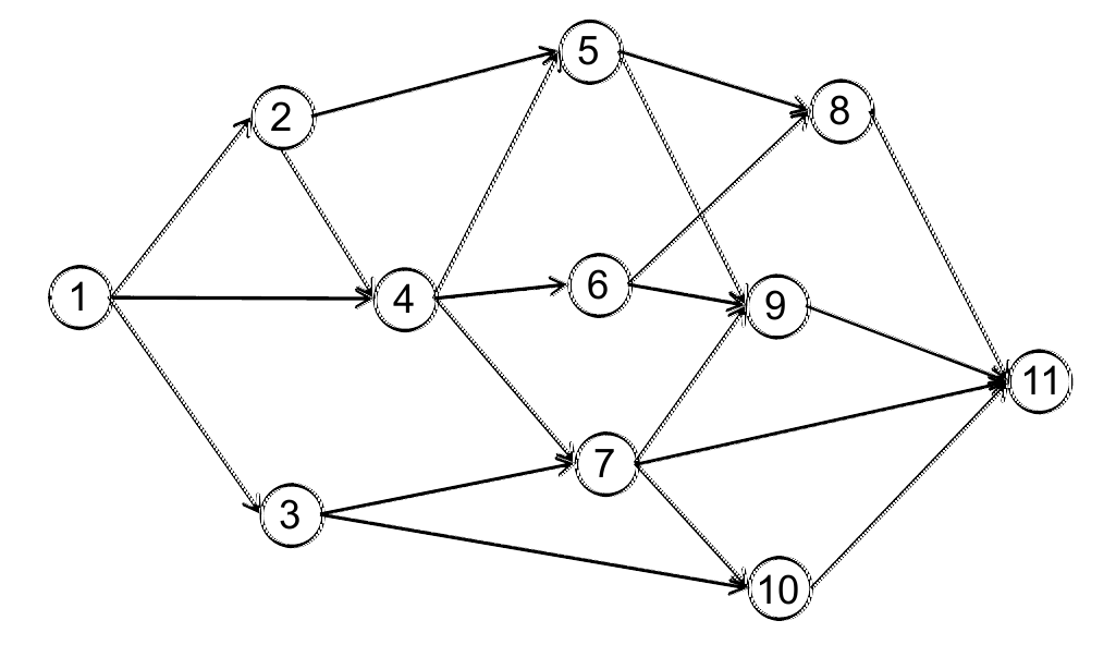
There are many problems where the transition from state $S_t$ to $S_{t+1}$ involves random information that is not known at time $t$. We saw a simple example of randomness in our first inventory problem, and a more complicated example in our second inventory problem.
For these more general problems, if we are in a state $S_t$, make a decision $x_t$, and then observe new information $W_{t+1}$ (that is not known at time $t$), it will take us to a new state $S_{t+1}$ according to our transition function
\[S_{t+1} = S^M(S_t,x_t,W_{t+1}).\]This means that at time $t$ when we have to choose $x_t$, $W_{t+1}$ is a random variable, which means that $S_{t+1}$ is a random variable as well. In this case we have to insert an expectation in Bellman’s equation and write equation $\eqref{eq:bellmangraph}$ as
\[\begin{align} V_t(S_t) = \max_{x_t} \big(C(S_t,x_t) + \E_{W_{t+1}} \left\{V_{t+1}(S_{t+1})\vert S_t,x_t\right\}\big). \label{eq:bellmanstochastic} \end{align}\]Here we have inserted the expectation $\E_{W_{t+1}}\lbrace \cdot\rbrace $ which literally means to average over all the random outcomes of $W_{t+1}$.
The stochastic version of Bellman’s equation in $\eqref{eq:bellmanstochastic}$ is extremely general. The state $S_t$ does not just mean a node in a graph; it captures any (and all) information relevant to the problem. The difficulty is that we can no longer compute the value function $V_t(S_t)$, which in turn means we will not have access to $V_{t+1}(S_{t+1})$ that we assumed we knew in equations $\eqref{eq:bellmangraph}$ and $\eqref{eq:bellmanstochastic}$.
The strategy the research community has used when trying to apply Bellman’s equation is to draw on the field of machine learning to estimate a statistical approximation that we are going to call $\Vbar_t(S_t)$. Assuming that we can come up with a reasonable approximation $\Vbar_{t+1}(S_{t+1})$, we would write our policy (our method for making a decision) using
\[\begin{align} X^\pi(S_t) = \argmax_{x_t\in\Xcal_t} \big(C(S_t,x_t) + \E_{W_{t+1}} \{\Vbar_{t+1}(S_{t+1})\vert S_t,x_t\}\big). \label{eq:introvbarpolicy} \end{align}\]The notation “$\argmax_x f(x)$” means the value of $x$ that maximizes the function $f(x)$. The index $\pi$ carries the information that specifies the structure of the function $f$, and any tunable parameters $\theta$ which we would need in the approximation $\Vbar_{t+1}(S_{t+1})$.
This class of policy falls under headings such as approximate dynamic programming and, most often, reinforcement learning. While a powerful idea, it is not easy to apply and depends on our ability to create an accurate approximation $\Vbar_{t+1}(S_{t+1})$.
There is a very rich literature on methods for approximating value functions, but it is no panacea. This book will illustrate this idea in a few places, but readers are cautioned that this class of policies is quite difficult to use.
-
4) Direct lookahead approximations (DLAs) – There are many problems where we simply cannot develop effective policies using any of the first three classes, and when this happens, we have to turn to direct lookahead approximations. We will write this out in its full mathematical form later, but for now, we are going to describe DLAs as making a decision now while optimizing over a (typically approximate) model that extends over some planning horizon.
A common DLA is to create an approximate model that is deterministic. This is what we are doing when we use a navigation system that finds the shortest path to the destination assuming that we know the travel time along each link of the network. As a general rule, solving an exact stochastic model of the future is almost always impossible, so we are going to investigate different strategies for approximating the problem.
We illustrated our modeling framework using two inventory problems, and suggested two simple policies (forms of PFAs) with equations $\eqref{eq:introorderupto}$ and $\eqref{eq:adjustedforecastpolicy}$, but we did this just to have a concrete example of a policy. While PFAs are widely used in day-to-day decision making, these are specialized examples.
By contrast, we are going to claim that the four classes of policies we just outlined (PFAs, CFAs, VFAs and DLAs) are universal, in that these cover any method that we might use to solve any sequential decision problem. To be clear, these are meta-classes. That is, if we think a problem lends itself to one particular class, we are not done, since we still have to design the specific policy within the class. Just the same, we feel that these four classes provide a roadmap to guide the process for designing policies.
Testing policies
To test the value of a policy, we are going to use equation $\eqref{eq:objectivecumulativerewardsample}$ which simulates a policy over a single sample path of the information process $W_t$. The hardest part when simulating a policy is typically creating the exogenous information process.
Let $\omega$ be a sample path, where $W_1(\omega), \ldots, W_T(\omega)$ represents a particular sample path. Table 1.3 illustrates 10 sample paths of prices that are indexed $\omega^1$ to $\omega^{10}$. If we choose $\omega^6$, then $W_7(\omega^6) = 44.16$.
| $t=1$ | $t=2$ | $t=3$ | $t=4$ | $t=5$ | $t=6$ | $t=7$ | $t=8$ | |
|---|---|---|---|---|---|---|---|---|
| $\omega^n$ | $p_1$ | $p_2$ | $p_3$ | $p_4$ | $p_5$ | $p_6$ | $p_7$ | $p_8$ |
| $\omega^1$ | 45.00 | 45.53 | 47.07 | 47.56 | 47.80 | 48.43 | 46.93 | 46.57 |
| $\omega^2$ | 45.00 | 43.15 | 42.51 | 40.51 | 41.50 | 41.00 | 39.16 | 41.11 |
| $\omega^3$ | 45.00 | 45.16 | 45.37 | 44.30 | 45.35 | 47.23 | 47.35 | 46.30 |
| $\omega^4$ | 45.00 | 45.67 | 46.18 | 46.22 | 45.69 | 44.24 | 43.77 | 43.57 |
| $\omega^5$ | 45.00 | 46.32 | 46.14 | 46.53 | 44.84 | 45.17 | 44.92 | 46.09 |
| $\omega^6$ | 45.00 | 44.70 | 43.05 | 43.77 | 42.61 | 44.32 | 44.16 | 45.29 |
| $\omega^7$ | 45.00 | 43.67 | 43.14 | 44.78 | 43.12 | 42.36 | 41.60 | 40.83 |
| $\omega^8$ | 45.00 | 44.98 | 44.53 | 45.42 | 46.43 | 47.67 | 47.68 | 49.03 |
| $\omega^9$ | 45.00 | 44.57 | 45.99 | 47.38 | 45.51 | 46.27 | 46.02 | 45.09 |
| $\omega^{10}$ | 45.00 | 45.01 | 46.73 | 46.08 | 47.40 | 49.14 | 49.03 | 48.74 |
Table 1.3. Illustration of a set of sample paths for prices all starting at $45.00.
The question is: how do we create a sample of observations such as those depicted in Table 1.3? There are three typical strategies:
- Create samples from historical data. Since there is only one outcome at any point in time, we can create multiple sample paths by combining observations from different periods of time. We might pick prices from different years, or demands from different months, or observed travel times on different days. This approach is not possible when the exogenous information depends on the state $S_t$ or decisions $x_t$.
- Simulating from a mathematical model. This approach offers the advantage of being able to generate large samples to get statistically reliable estimates of the performance of a policy. These models can be very sophisticated, but it is quite easy to create models (even sophisticated ones) that do not replicate the behavior of real data. The biggest challenge is capturing correlations, either over time or between samples (say the demands of different products, the prices of different stocks, or the wind speed in different locations).
- We can test an idea in the field, using observations as they actually occur. The advantage of this is that we are working with real data (history may not be the same as the future). The disadvantage is that it takes a day to observe a day of new data (and we may need much more than a single day of observations).
If $W_{t+1}$ depends on the state $S_t$ and/or decision $x_t$, then we have to devise a way to reflect this dependence. Creating a mathematical model makes it possible to perform many simulations in the computer, but creating samples of the information process also requires recreating correlations across time, as well as over space. We refer the reader to RLSO, Chapter 10, for a more in-depth discussion of uncertainty modeling.
Next steps
The next five chapters of the book are going to apply our modeling framework to five different problems:
- Chapter 2 – An asset selling problem
- Chapter 3 – Adaptive market planning
- Chapter 4 – Learning the best diabetes medication
- Chapter 5 – Stochastic shortest path problems - Static
- Chapter 6 – Stochastic shortest path problems - Dynamic
Each of these chapters will follow the same outline as we used above to describe the two inventory problems. This outline consists of:
- Narrative – A plain English description of the problem.
- The universal model – This model will follow our format of describing the five elements of a sequential decision problem: state variables, decision variables, exogenous information variables, the transition function and the objective function.
- Uncertainty model – Here we will provide a possible model of any uncertainties in the problem.
- Designing policies – We are going to suggest possible policies for making decisions. We have chosen our problems so that the five application settings will give us a tour through all four classes of policies. For now, we are going to let the reader try to recognize which of the four classes we are choosing.
- Extension – Finally we may suggest one or more possible extensions of our basic problem that may require changing the policy.
We then return to the four classes of policies in Chapter 7 and discuss our general modeling framework, using the problems in Chapters 2–6 to illustrate different modeling ideas.
After this discussion, we return to our pattern of teach-by-example chapters, but using more complex problems. Our remaining chapters cover the following problems:
- Chapter 8 – Energy storage I
- Chapter 9 – Energy storage II
- Chapter 10 – Supply chain management I: The two-agent newsvendor
- Chapter 11 – Supply chain management II: The beer game
- Chapter 12 – Ad-click optimization
- Chapter 13 – Blood management problem
- Chapter 14 – Optimizing clinical trials
What did we learn?
- To begin, we learned what a decision is!
- We presented a general model, called the universal modeling framework, for any sequential decision problem.
- We illustrated the model by first using a classical inventory problem, where the state of the system is the amount in inventory.
- We then transitioned to a slightly more complicated inventory problem where the state variable includes the resource state $R_t$ of inventory, an informational state variable in the form of price $p_t$, and finally a belief state about the upcoming demand $\Dhat_{t+1}$ in the form of an estimated mean and variance.
- We learned how to model the flow of exogenous information that may arrive from a number of different sources. Exogenous information is represented as a function that might depend on the state and/or the decision.
- We illustrated two forms of a simple class of policy known as a policy function approximation (or PFA).
- We learned that policies can be evaluated in a number of different ways that depend on the context and how decisions are used.
- We closed with a brief overview of four classes of policies. Illustrations of all four classes will be provided in Chapters 2–6, at which point we pause in Chapter 7 to discuss the policies in greater depth, setting the stage for the more complex problems in Chapters 8–14.
Exercises
Review questions
- What are the five elements of the mathematical model of a sequential decision problem?
- What is the difference between the variables in the initial state $S_0$ and those in the dynamic state $S_t$ for $t > 0$?
- What is the difference between a decision and the exogenous information?
- What are the two major categories of policies, and how are they different?
- Compare the state variables for the simple inventory problem to the more complicated inventory problem.
Problem solving questions
- Compare the policies for the two inventory problems in terms of how they would handle time-dependent behavior. For example, our pizza parlor may have much higher demands on weekends than on weekdays. Comment on the value of making the tunable parameter $\theta$ time-dependent (or day of week dependent) in terms of how it might improve the solution.
- Contrast how you might go about tuning the parameter $\theta$ for the inventory problems:
- In a simulator.
- In the field.