Chapter 6: Stochastic shortest path problems - Dynamic

Chapter overview

Chapter 5 posed a shortest path problem which assumes we either do not know anything about dynamically changing travel times on links, or we may observe the times on links that are connected to the intersection where our traveler is located (but nothing further in the future).

Now imagine that we are a service like Google maps that has access to real-time information over the entire network. Further, this information is being updated in real time which leads to Google updating the recommended path to the traveler’s destination. This information introduces a major change into the model which completely eliminates any possibility of using the methods that we presented in Chapter 5.

The approach we use for this problem applies to any problem that we would solve by planning into the future using what might be called “best estimates” of uncertain values. This provides a setting for our first use of the fourth class of policy which we call direct lookahead approximations. We use this setting to demonstrate a practical and powerful method for making decisions in a dynamic setting (which means under uncertainty) where we start with a deterministic lookahead model, and then introduce parameters to make it work better over time, under uncertainty.

Narrative

We are going to tackle stochastic shortest paths again, but this time we are going to do it just as it is done in Google maps (or any commercial navigation system). We all recognize that transportation networks often have predictable patterns of congestion, along with random variations that happen in the natural course of events. For example, an accident might create a backlog where we might estimate how the travel delays might evolve as a result of the accident.

The point of departure from the static shortest path problem is that our estimates of costs in the future are evolving over time. We are going to return to the problem where costs are stochastic, but when we arrive at a node $i$, we do not see the actual realizations of the costs out of node $i$. However, we are going to assume that we are given updated estimates of costs over the entire network. These estimates can be viewed as a forecast; we are going to assume that the actual cost that we incur when we traverse an arc will, on average, equal the forecast (that is, the forecasts are unbiased), but these forecasts will evolve over time as we get updates on the status of the network.

Framing the problem

The answers to our three framing questions are:

• Metrics: We wish to minimize the expected travel time, where we may also include a penalty for arriving after a target arrival time.
• Decisions: For a traveler at node $i$, we want to tell him which node $j$ to traverse to next.
• Uncertainties: The estimated travel times change randomly each time a traveler traverses a link to a downstream node. The actual time when traversing a link will differ from the estimate.

Basic model

Assume that when we have to make a decision at time $t$, we have an updated estimate of travel costs based on current congestion levels (by tracking the speed at which our smartphones are moving through traffic). We are going to represent these times using $\cbar_{tk\ell}$, the estimated cost of traversing link $(k,\ell)$ at time $t$, using estimates based on what we know at time $t$.

For now, we are not going to try to model the cost if we arrive at a point in time $t’ > t$ given what we know at time $t$. So, we may estimate, at 3pm, that we are going to arrive at a link at 5pm, but we are going to use our 3pm estimate (as Google does now).

State variables

A traveler at node $N_t = i$ at time $t$ is assumed to be given a set of forecasts $\cbar_{t} = (\cbar_{ttk\ell})_{k, \ell \in \Ncal}$, the vector of estimates of the cost to traverse link $(k, \ell)$ at time $t$, given what is known at time $t$. The traveler’s state $S_t$ at time $t$ is then

Note that this state variable is very large; it consists of a vector of estimates of link costs for every link in the network.

Decision variables

The decision variables are the same as with the static stochastic shortest path problem

This decision has to obey the constraint that we do something when we are in state $N_t = i$ as long as $i$ is not the destination. We write this constraint as

If we are at the destination, then we do nothing, and instead write $x_{tij} = 0$ for $i$ equal to the destination, and $j$ any other node.

As above, we let $X^\pi(S_t)$ be our policy for determining the vector $x_t$ which we assume has to satisfy the constraint $\eqref{dynamicshorestpathconstraint}$.

Exogenous information

There are two types of exogenous information for this problem. The first type is the observed costs: $\chat_{t+1,ij}$, the actual cost of traversing link $(i,j)$ after the traveler made the decision at time $t$ to traverse this link. Note that we only observe $\chat_{t+1,ij}$ if the traveler traverses link $(i,j)$ (we can just insert 0 for links we do not traverse, since we will not use these values).

The second type of new information is the updates to the estimates $\cbar_t$ of the link costs. We are going to model the exogenous information as the change in the estimates:

Our exogenous information variable, then, is given by

Transition function

We are assuming that $\chat_{t+1}$ arrives as exogenous information (we could have let the exogenous information be the change in the costs, but this is more natural).

The transition function for the forecasts evolves according to

Finally, we update the physical state $N_t$ using

In other words, if we are at node $i=N_t$ and we make the decision $x_{tij}= 1$ (which requires that we be at node $i$, since otherwise $x_{tij} = 0$), then $N_{t+1} = j$.

The updating of $\chat_{t+1}$, equation $\eqref{eq:shortestpathdynamictransition1}$ for the forecasts $\cbar_{t+1}$ and equation $\eqref{eq:shortestpathdynamictransition2}$ for our physical state $R_t$, make up our transition function

Objective function

We now write our objective function as

Note that our policy $X^\pi(S_t)$ makes the choice of the next link we move to given what we know at time $t$, captured by $S_t$.

Modeling uncertainty

In practice, the dynamic updating of costs (and forecasts) come from real systems, which means they are data driven. When this is the case, we do not use a mathematical model of the link costs. The alternative is to have a mathematical model of the random information $W^{n+1}$.

If we wish to run simulations, then we face the challenge of modeling the realization of the costs captured by $\chat_t$, as well as the sequence of forecasts. Considerable care has to be given to this model. First, the change in the estimate of $\ctilde_t$, which we represent by $\delta \ctilde_{t+1}$, has to be drawn from a distribution with mean $0$. In addition, the realizations $\chat_{t+1}$ have to be drawn from a distribution with mean $\ctilde_t$.

We do not want to minimize the challenge of creating a realistic stochastic model. Changes in link costs arise from different sources, from natural traffic variations, weather, accidents, and shifts in flows due to drivers responding to congestion elsewhere in the network. Stochastic variations in link costs are nonstationary, and are not independent, either over time or across links. However, beyond recognizing the difficult challenges, a more realistic model is beyond the scope of our discussion.

Designing policies

A quick hint that we are not going to be using Bellman’s equation (even approximately) is the size of the state variable, which now includes forecasts of travel costs on every link in the network.

Instead, we are going to base our policy on a special model that we call a lookahead model. For example, at time $t$ we can create a model consisting of states $S_t$, decisions $x_t$ and exogenous information $W_{t+1}$, but in our base problem the state variable $S_t = (N_t, \cbar_t)$, which is quite complicated.

Instead, we are going to create a simpler model where we first create a new set of variables that are typically approximations of the variables in the base model. We differentiate a new set of variables for our lookahead models by putting tildes on the variables in the lookahead model, and index them by two time indices: time $t$, which is the time at which a decision is being made, and a second index $t’$ which is the time within the lookahead model.

The sequence of states, decisions and exogenous information in the lookahead model would then be written

Our vector of costs $\cbar_t$ would then be replaced with the vector $\ctilde_{tt’}$. We now face the challenge of designing a lookahead policy that we could call $\Xtilde_{tt’}(\Stilde_{tt’})$ that determines $\xtilde_{tt’}$ within the lookahead model. Below we propose two strategies, both of which can be solved using a simple shortest path algorithm.

A deterministic lookahead policy

We approximate the problem by assuming that the costs in the lookahead model, $\ctilde_{tt’}$, are fixed and equal to the current estimates which means we let

This means that we no longer have the exogenous information variables $\Wtilde_{tt’}$, which gives us a deterministic lookahead model.

This allows us to solve our lookahead model deterministically, treating the cost estimates $\ctilde_{tt’,k\ell}$ as the correct cost rather than random variables. In this case, our state variable is once again simply the node where the traveler is located (within the lookahead model).

We can solve this problem with a standard shortest path algorithm which, as we saw in Chapter 5, is a deterministic dynamic program that we can solve with Bellman’s equation, which we do by first finding the “value” of being at node $i$ at time $t’$ in our lookahead model. We can compute these values by setting the values at the end of our lookahead model for time $t$ equal to zero

Then, we step back in time (in the lookahead model) for $t’ = t+H-1, t+H-2, \ldots, t$ and compute, for each node $i$:

Our lookahead policy is then given by

Finally, the policy that we are going to implement in the base model, if we are at node $i$, would be

This is the policy that we are using when we follow a navigation system. Making decisions based on a deterministic lookahead model is one of the most widely used methods for making decisions in sequential decision problems under uncertainty.

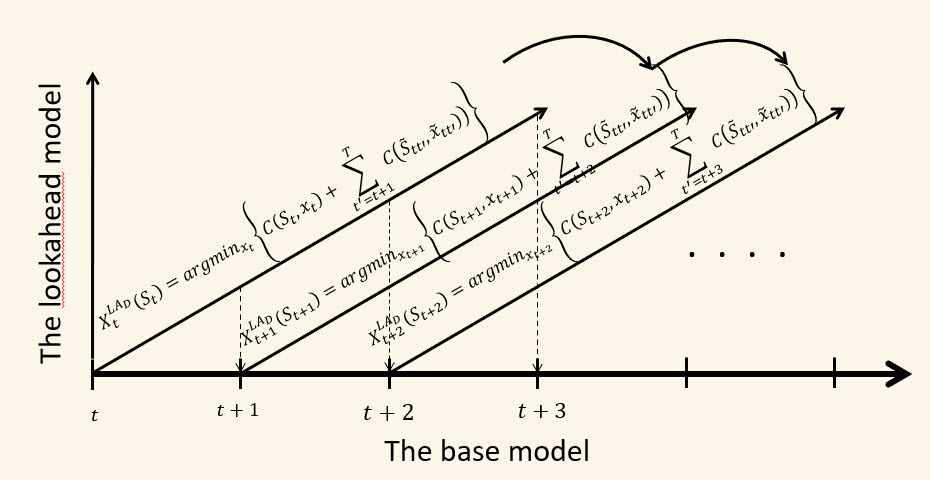
Figure 6.1 illustrates a rolling lookahead process. At times $t$, $t+1$, $t+2$, $\ldots$, we create and solve a lookahead model using estimates of costs as we know them. We then solve our shortest path problem, which is represented in the decisions $\xtilde_{tt’}(j)$ for all nodes $j$, but then we only implement the decision $\xtilde_{tt}(i)$ for the node $i$ where we are located at time $t$.

When we hold a dynamically changing variable constant in a lookahead model, we refer to this variable as a latent variable in the lookahead model. The term “latent variable” technically means hidden variable; in this context it refers to a variable that is not changing over time (within the lookahead model), in which case we drop it from the state variable, which means it is hidden (again, in the lookahead model).

This is one of a number of different types of approximations that can be made in a lookahead model. The most obvious approximation we are making is that we use a deterministic future which means that the estimates of link costs are being held constant within the lookahead model, even while they are changing in the base model.

The lookahead model, then, is its own model with its own characteristics, which is the reason why we use variables with tildes — this is how we make the distinction between our base model, which uses variables such as $S_t$ and $x_t$, and the lookahead model, where we use variables such as $\Stilde_{tt’}$ and $\xtilde_{tt’}$.

Next, we are going to propose a minor tweak to make this approach work better under uncertainty.

A parameterized deterministic lookahead policy

A simple strategy for handling uncertainty in our dynamic shortest path problem would be to replace our point estimate $\ctilde_{tt’k\ell}=\cbar_{tk\ell}$ for the cost of traversing link $(k,\ell)$ at time $t$ with, say, the $\theta$-percentile of the costs, suggesting that we write the costs as $\ctilde_{tt’,k\ell}(\theta) = \cbar_{tij}(\theta)$. This logic could, for example, avoid a path through an area that sometimes becomes very congested, where the cost might be quite high.

This policy still produces a deterministic shortest path problem which is as easy to solve as when we used the point estimates $\cbar_t$. We simply modify equations $\eqref{eq:shortestpathdetlookahead}$–$\eqref{eq:shortestpathbellmandetlookahead}$ above by using the $\theta$-percentile link costs. We then designate the value functions $\Vtilde_{tt’}(i\vert \theta)$ to indicate the dependence on the parameter $\theta$, which is computed using

Our lookahead policy is then given by

We then write our parameterized policy for the base model (which gives the decisions that are actually implemented) using

This is equivalent to our original deterministic lookahead model, with one major exception: we need to tune $\theta$ by optimizing

where $S_{t+1} = S^M(S_t,X^\pi(S_t\vert \theta), W_{t+1})$ (see equations $\eqref{eq:shortestpathdynamictransition1}$–$\eqref{eq:shortestpathdynamictransition2}$) using some method for generating random realizations of $W_1, \ldots, W_T$.

The optimization problem in $\eqref{eq:tuneshortestpathcfa}$ is itself a challenging problem, but it is helped because $\theta$ is a scalar between 0 and 1. Practical algorithms for optimizing the objective function in $\eqref{eq:tuneshortestpathcfa}$ typically involve running simulations to get noisy observations of the function.

An obvious question is whether the use of a percentile different than $\theta = 0.5$ would improve the results. Our experience is that this is true when there is a penalty for late arrivals (for example, we want to arrive for an appointment at 9am).

What did we learn?

• We showed how to model a dynamic network problem, where the estimates of costs evolve over time. This time, the state of the system is the location of the traveler along with the estimates of costs on every link in the network.
• We introduced the idea of an approximate lookahead model, in this case a deterministic lookahead, which can be solved as a shortest path problem. Although this is an optimal solution, solving an approximate lookahead model, even optimally, is not an optimal policy.
• We describe latent variables, which are dynamic variables (the costs on the links) that are held constant in the lookahead model (which is why they are no longer in the state variable).
• We show how we can modify our deterministic lookahead into a parameterized deterministic lookahead. Instead of using the expected cost on each link, we might use the $\theta$-percentile so that we consider how bad a link might be. The parameter $\theta$ has to be tuned, making this a hybrid of a deterministic lookahead approximation (a DLA policy) that is parameterized, which makes it a form of CFA policy, giving us a hybrid DLA/CFA policy.

Exercises

Review questions

1. Why couldn't we use the approximate dynamic programming methods of [Chapter 5](/sdam/chapter-5/) to solve our dynamic problem?
2. How are we modeling the exogenous process $W_t$, in the lookahead model?
3. Describe in words what we mean by a lookahead policy.

Problem solving questions

1. We solve a deterministic lookahead model as our policy. This solves the deterministic problem optimally. Why isn't this an optimal policy?
2. We solve our deterministic lookahead model (possibly with modified costs $\cbar_{ij}(\theta)$) as a deterministic dynamic program using Bellman's equation. Why wouldn't we then say that we are solving our base model using dynamic programming?
3. Imagine that we want to leave as late as possible from the origin node, but there is a high penalty for arriving late at the destination. If we optimize over the $\theta$-percentile of the costs $\cbar_{tij}(\theta)$, how might this logic help us avoid late arrivals?
4. Given the insights from exercise 6, how do you think using the $\theta$-percentile costs would help for a problem where we are simply trying to minimize total travel time without regard to the possibility of arriving late?
5. Provide the full model (state variables, decision variables, ...) for the setting where costs $\chat_{tij}$ on links out of node $i$ are revealed when the traveler arrives at node $i$ and before she makes a decision which link to traverse. Remember that you are minimizing cumulative costs over the path. You do not have to design a policy; follow our standard practice of introducing a policy $X^\pi(S_t)$ without specifying the policy.
6. Imagine that we want to solve our shortest path problem where we want to depart as late as possible from the origin, but we need to arrive to the destination by 9am. We assess a penalty $\eta$ for each minute we arrive after 9am. Describe a base model and parameterized lookahead policy for solving this problem. What is the state variable for the base model? What is the state variable for the lookahead model?

Programming questions

These exercises use the Python module StochasticShortestPath_Dynamic on tinyurl.com/sdagithub.

1. We are going to use a deterministic lookahead model as was done in the notes, but instead of using the expected cost on each link, we are going to use a percentile that we designate by $\theta^{cost}$. For example, if $\theta^{cost} = 0.8$, then we would use the 80th percentile of the cost (think of this as using an estimate of how large the cost might be). Let $\cbar_{tij}(\theta^{cost})$ be the $\theta^{cost}$-percentile cost of link $(i,j)$ given what we know at time $t$.
   1. Write out the lookahead model, which would be a deterministic shortest path using costs $\cbar_{tij}(\theta^{cost})$ (as is done in the book). Use this model to formally define a lookahead policy $X^{DLA}(S_{tj}\vert \theta^{cost})$.
   2. What is the state variable for the dynamic problem? Remember that the state variable includes all dynamically varying information used to make a decision (which includes computing costs and constraints), as well as computing the transition from $t$ to $t + 1$.
   3. Write out the objective function used to evaluate our lookahead policy.
   4. We now have a policy $X^{DLA}(S_{tj}\vert \theta^{cost})$ parameterized by $\theta^{cost}$. Using the python module StochasticShortestPath_Dynamic, simulate the policy for $\theta^{cost} = (0, 0.1, 0.2, 0.3, 0.4, 0.5, 0.6, 0.7, 0.8, 0.9, 1.0)$. Simulate each version of the policy 100 times and take an average of the total actual cost (not the $\theta^{cost}$-percentile). Also consider the risk of being "late," i.e., the total actual cost being greater than a given threshold. Plot the results and compare them.