Chapter 13: Blood management problem
Chapter overview
The blood management problem is a multidimensional resource allocation problem since we have to manage eight different blood types, while also keeping track of how long blood has been stored (unless it is frozen). This is the first time we have to draw on tools like linear programming to make decisions at each point in time.
We start by illustrating a myopic policy that involves solving a simple linear program which ignores making decisions that do not understand the impact of decisions now on the future. For blood management, that can arise in the management of $O-$ blood, which is known as the universal donor – it can be used for any patient. It helps to hold reserves of $O-$ blood in case there is a shortage of other types.
We then demonstrate the use of approximate dynamic programming to balance rewards now with rewards in the future. To use ADP for a multidimensional problem, we take advantage of the structure of the problem in the design of an approximation for the value of a set of blood inventories in the future. This idea works when we can exploit the structure of the problem.
Narrative
The problem of managing blood inventories serves as a particularly elegant illustration of a resource allocation problem. We are going to start by assuming that we are managing inventories at a single hospital, where each week we have to decide which of our blood inventories should be used for the demands that need to be served in the upcoming week.
We have to start with a bit of background about blood. For the purposes of managing blood inventories, we care primarily about blood type and age. Although there is a vast range of differences in the blood of two individuals, for most purposes doctors focus on the eight major blood types: $A+$ (“A positive”), $A-$ (“A negative”), $B+$, $B-$, $AB+$, $AB-$, $O+$, and $O-$. While the ability to substitute different blood types can depend on the nature of the operation, for most purposes blood can be substituted according to Table 13.1.
| Donor \ Recipient | $AB+$ | $AB-$ | $A+$ | $A-$ | $B+$ | $B-$ | $O+$ | $O-$ |
|---|---|---|---|---|---|---|---|---|
| $AB+$ | X | |||||||
| $AB-$ | X | X | ||||||
| $A+$ | X | X | ||||||
| $A-$ | X | X | X | X | ||||
| $B+$ | X | X | ||||||
| $B-$ | X | X | X | X | ||||
| $O+$ | X | X | X | X | ||||
| $O-$ | X | X | X | X | X | X | X | X |
Table 13.1. Allowable blood substitutions for most operations, "X" means a substitution is allowed.
A second important characteristic of blood is its age. The storage of blood is limited to six weeks, after which it has to be discarded. Hospitals need to anticipate if they think they can use blood before it hits this limit, as it can be transferred to blood centers which monitor inventories at different hospitals within a region. It helps if a hospital can identify blood it will not need as soon as possible so that the blood can be transferred to locations that are running short.
Framing the problem
The answers to our three framing questions are:
- Metrics: Maximize the expected sum of bonuses minus penalties for allocating blood of one type to satisfy demand of another type.
- Decisions: How much blood of one type to assign to demands for blood of another type, along with how much blood to hold in inventory for each blood type.
- Uncertainties: The future demands for blood of each type, along with the donations of each blood type.
Basic model
State variables
We can model the blood problem as a heterogeneous resource allocation problem. We are going to start with a fairly basic model which can be easily extended with almost no notational changes. We begin by describing the attributes of a unit of stored blood using
\[b = \begin{pmatrix} b_1 \\ b_2 \end{pmatrix} = \begin{pmatrix} \text{blood type } (A+, A-, \ldots) \\ \text{age (in weeks)} \end{pmatrix},\]and let $\Bcal$ be the set of all blood attribute types. We will limit the age to the range $0 \leq b_2 \leq 6$. Blood with $b_2 = 6$ (which means blood that is already six weeks old) is no longer usable. We assume that decision epochs are made in one-week increments. Blood inventories are represented using $R_{tb}$, the units of blood of type $b$ available to be assigned or held at time $t$, with $R_t = (R_{tb})_{b\in\Bcal}$.
The attributes of demand for blood are given by
\[a = \begin{pmatrix} a_1 \\ a_2 \\ a_3 \end{pmatrix} = \begin{pmatrix} \text{blood type of patient} \\ \text{surgery type: urgent or elective} \\ \text{is substitution allowed?} \end{pmatrix},\]and let $\Acal$ be the set of all attribute types for blood demands. The attribute $a_3$ captures the fact that there are some operations where a doctor will not allow any substitution. One example is childbirth, since infants may not be able to handle a different blood type, even if it is an allowable substitute. For our basic model, we do not allow unserved demand in one week to be held to a later week.
We then define the demand for blood using $D_{ta}$, the number of units of blood required for patients with attribute $a$ at time $t$, with $D_t = (D_{ta})_{a\in\Acal}$.
The state variables are given by
\[S_t = (R_t,D_t).\]Decision variables
We act on blood resources with decisions given by $d$, a type of decision, which includes decisions to give blood to a patient with attribute $a\in\Acal$, or to do nothing and hold the blood, which we represent by $d^\phi$; and $\Dcal$, the set of all possible decisions, $\Dcal = \Acal \cup d^\phi$.
We then let $x_{tbd}$ be the number of units of blood with attribute $b$ that we act on with a decision of type $d$ at time $t$, with $x_t = (x_{tbd})_{b\in\Bcal,d\in\Dcal}$.
The feasible region $\Xcal_t$ is defined by the following constraints:
\[\begin{align} \sum_{d\in\Dcal} x_{tbd} &= R_{tb}, \quad b\in\Bcal, \label{eq:blood1}\\ \sum_{b\in\Bcal} x_{tbd} &\leq \Dhat_{td}, \quad d\in\Dcal,\label{eq:blood2}\\ x_{tbd} &\geq 0. \label{eq:blood3} \end{align}\]Exogenous information
The information that arrives after we have made a decision is given by the blood donations which we represent using $\Rhat_{t+1,b}$, the number of new units of blood of type $b$ donated between $t$ and $t+1$, with $\Rhat_{t+1} = (\Rhat_{t+1,b})_{b\in\Bcal}$.
The new demands for blood are modeled using $\Dhat_{t+1,a}$, the units of demand with attribute $a$ that arose between $t$ and $t+1$, with $\Dhat_{t+1} = (\Dhat_{t+1,a})_{a\in\Acal}$.
Our exogenous information variable would be
\[W_{t+1} = (\Rhat_{t+1}, \Dhat_{t+1}).\]Transition function
Blood that is held simply ages one week, but we limit the age to six weeks. Blood that is assigned to satisfy a demand can be modeled as being moved to a blood-type sink, denoted, perhaps, using $b_{t,1} = \phi$ (the null blood type). The blood attribute transition function $b^M(b_t,d_t)$ is given by
\[b_{t+1} = \begin{pmatrix} b_{t+1,1} \\ b_{t+1,2} \end{pmatrix} = \begin{cases} \begin{pmatrix} b_{t,1} \\ \min\{6,b_{t,2}+1\} \end{pmatrix}, & d_t = d^\phi, \\[8pt] \begin{pmatrix} \phi \\ - \end{pmatrix}, & d_t \in\Dcal. \end{cases}\]To represent the transition function, it is useful to define
\[\delta_{b'}(b,d) = \begin{cases} 1 & b^x_t = b' = b^M(b_t,d_t),\\ 0 & \text{otherwise,} \end{cases}\]and let $\Delta$ be the matrix with $\delta_{b’}(b,d)$ in row $b’$ and column $(b,d)$.
We note that the attribute transition function is deterministic. A random element would arise, for example, if inspections of the blood resulted in blood that was less than six weeks old being judged to have expired. The resource transition function can now be written as
\[R^x_{tb'} = \sum_{b\in\Bcal}\sum_{d\in\Dcal} \delta_{b'}(b,d) x_{tbd}, \qquad R_{t+1,b'} = R^x_{tb'} + \Rhat_{t+1,b'}.\]In matrix form, these would be written as
\[\begin{align} R^x_t &= \Delta x_t, \label{eq:bloodresourcetransition1}\\ R_{t+1} &= R^x_t + \Rhat_{t+1}. \label{eq:bloodresourcetransition2} \end{align}\]The demands $D_{t+1}$ are simply observed from the new demands $\Dhat_{t+1}$, so we write this as
\[D_{t+1} = \Dhat_{t+1}.\]Figure 13.1 illustrates the transitions that are occurring in week $t$. We either have to decide which type of blood to use to satisfy a demand (Figure 13.1a), or to hold the blood until the following week. If we use blood to satisfy a demand, it is assumed lost from the system. If we hold the blood until the following week, it is transformed into blood that is one week older. Blood that is six weeks old may not be used to satisfy any demands, so we can view the bucket of blood that is six weeks old as a sink for unusable blood (the value of this blood would be zero). Note that blood donations are assumed to arrive with an age of 0.
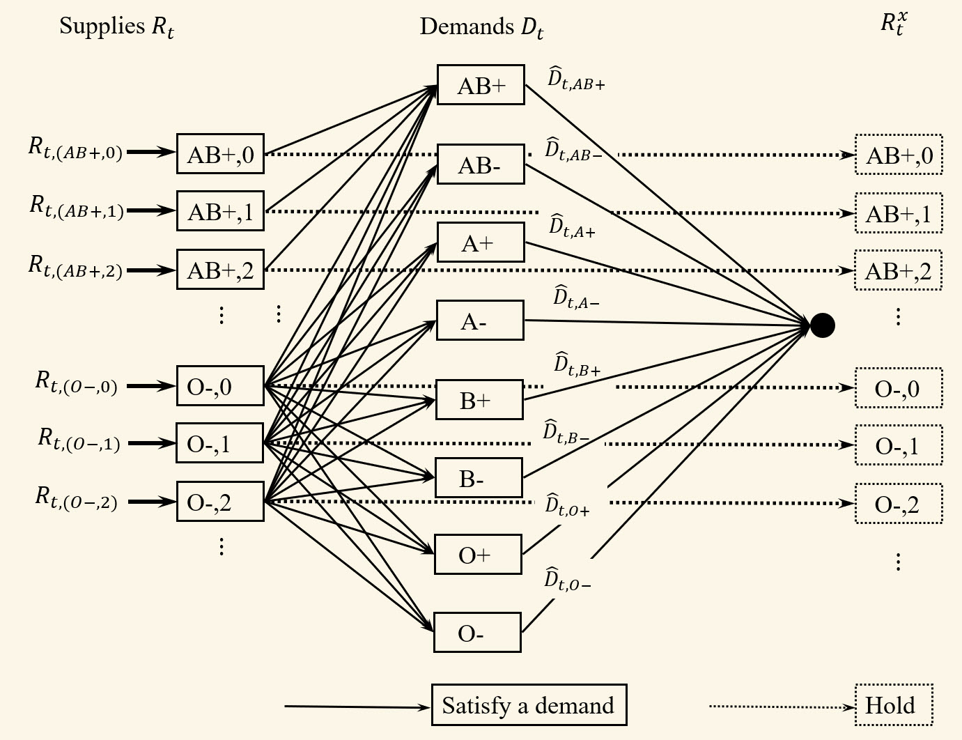
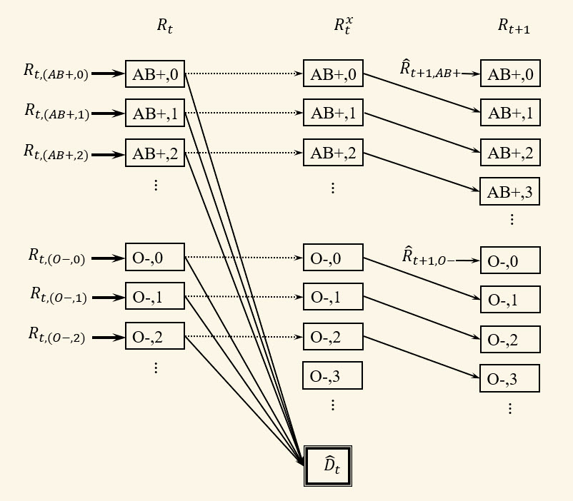
The models represented by Figure 13.1 are quite useful for resource allocation problems. We have used this model quite successfully to optimize the allocation of manufactured products across distribution centers, and to optimize the allocation of trucks, freight cars and locomotives in freight transportation. Care has to be used when estimating the value function approximations, but once they are estimated, their use produces sequences of very small network problems that are shown in the figure.
Objective function
There is no real “cost” to assigning blood of one type to demand of another type (we are not considering steps such as spending money to encourage additional donations, or transporting inventories from one hospital to another). Instead, we use the contribution function to capture the preferences of the doctor. We would like to capture the natural preference that it is generally better not to substitute, and that satisfying an urgent demand is more important than an elective demand.
For example, we might use the contributions described in Table 13.2. Thus, if we use $O-$ blood to satisfy the needs for an elective patient with $A+$ blood, we would pick up a -$10 contribution (penalty since it is negative) for substituting blood, a +$5 for using $O-$ blood (something the hospitals like to encourage), and a +$20 contribution for serving an elective demand, for a total contribution of +$15.
| Condition | Description | Value |
|---|---|---|
| if $d = d^\phi$ | Holding | 0 |
| if $b_1 = b_1$ when $d\in\Dcal$ | No substitution | 0 |
| if $b_1 \neq b_1$ when $d\in\Dcal$ | Substitution | -10 |
| if $b_1 = O-$ when $d\in\Dcal$ | $O-$ substitution | 5 |
| if $d_2 = $ Urgent | Filling urgent demand | 40 |
| if $d_2 = $ Elective | Filling elective demand | 20 |
Table 13.2. Contributions for different types of blood and decisions.
The total contribution (at time $t$) is finally given by
\[C_t(S_t,x_t) = \sum_{b\in\Bcal}\sum_{d\in\Dcal} c_{tbd} x_{tbd}.\]As before, let $X^\pi_t(S_t)$ be a policy (some sort of decision rule) that determines $x_t\in\Xcal_t$ given $S_t$. We wish to find the best policy by solving
\[\begin{align} \max_{\pi\in\Pi} \E \sum_{t=0}^T C_t(S_t,X^\pi(S_t)), \label{eq:bloodobjective} \end{align}\]where $S_{t+1} = S^M(S_t,X^\pi(S_t),W_{t+1})$.
Modeling uncertainty
The sources of uncertainty in this problem are blood donations, and the arrival of new surgeries requiring blood donations. Some issues we need to consider when modeling this uncertainty include:
- Not only is there randomness in the number of units of blood being donated, but also the type of blood.
- There are both day-of-week and seasonal patterns to blood donations, as well as responses to appeals which, of course, represent a decision.
- The arrival of new surgeries can come in bursts due to weather or violence.
- There is a consistent mismatch between the types of people who donate blood, and the types of people who need surgeries, which emerges in differences in the distribution of blood types.
- A major issue is managing the substitution of blood types. A lot of attention is given to the ability to use $O-$ blood for anyone, but there are different types of substitution for all blood types.
Designing policies
We are going to start with a basic myopic policy, and then transition to one that depends on approximating the value of blood inventories in the future.
A myopic policy
The most obvious way to solve this problem is a simple myopic policy, where we maximize the contribution at each point in time without regard to the effect of our decisions on the future. We can obtain a family of myopic policies by adjusting the one-period contributions.
For example, our bonus of $5 for using $O-$ blood (in Table 13.2), is actually a type of myopic policy. We encourage using $O-$ blood since it is generally more available than other blood types. By changing this bonus, we obtain different types of myopic policies that we can represent by the set $\Pi^M$, where for $\pi\in\Pi^M$ our decision function would be given by
\[\begin{align} X^\pi_t(S_t) = \argmax_{x_t\in\Xcal_t} \sum_{b\in\Bcal} \sum_{d\in\Dcal} c_{tbd}x_{tbd}. \label{eq:bloodmyopic} \end{align}\]The optimization problem in $\eqref{eq:bloodmyopic}$ is a simple linear program. Searching over policies in the optimization problem given by equation $\eqref{eq:bloodobjective}$ means searching over different values of the bonus for using $O-$ blood.
A VFA policy
As a traditional dynamic program, the optimization problem posed in equation $\eqref{eq:bloodobjective}$ is quite daunting. The state variable $S_t$ has $\vert \Acal\vert + \vert \Bcal\vert = 8 \times 6 + 8 \times 2 \times 2 = 80$ dimensions. The random variables $\Rhat$ and $\Dhat$ also have a combined 80 dimensions. The decision vector $x_t$ has $27 + 8 = 35$ dimensions.
It is natural to use value function approximations to determine the allocation vector $x_t$ using
\[\begin{align} x^n_t = \argmax_{x_t\in\Xcal^n_t} \big(C_t(S^n_t,x_t) + \Vbar^{x,n-1}_t(R^x_t) \big), \label{eq:adpblood} \end{align}\]where $R^x_t = R^M(R_t,x_t)$ is given by equation $\eqref{eq:bloodresourcetransition1}$ and where $\Xcal^n_t$ is defined by the constraints $\eqref{eq:blood1}$–$\eqref{eq:blood3}$. The key constraint is $\eqref{eq:blood1}$ which limits the availability of blood supplies of each type.
The first (and most important) challenge we face is identifying an appropriate approximation strategy for $\Vbar^{x,n-1}_t(R^x_t)$. A simple and effective approximation is to use separable, piecewise linear approximations, which is to say
\[\Vbar^x_t(R^x_t) = \sum_{b\in\Bcal} \Vbar^x_{tb}(R^x_{tb}),\]where $\Vbar^x_{tb}(R^x_{tb})$ is a scalar, piecewise, linear function in the post-decision inventory $R^x_{tb}$ for each blood type $b$.
It is easy to show that the value function is concave (as well as piecewise linear), so each $\Vbar^x_{tb}(R^x_{tb})$ should also be concave. Without loss of generality, we can assume that $\Vbar^x_{tb}(R^x_{tb}) = 0$ for $R^x_{tb} = 0$, which means the function is completely characterized by its set of slopes. We can write the function using
\[\begin{align} \Vbar^{n-1}_{tb}(R^x_{tb}) = \left(\sum_{r=1}^{\lfloor R^x_{tb}\rfloor} \vbar^{n-1}_{tb}(r-1) + (R^x_{tb} - \lfloor R^x_{tb}\rfloor) \vbar^{n-1}_{tb}(\lfloor R^x_{tb}\rfloor)\right), \label{eq:pwl} \end{align}\]where $\lfloor R \rfloor$ is the largest integer less than or equal to $R$. As we can see, this function is determined by the set of slopes $(\vbar^{n-1}_{tb}(r))$ for $r = 0, 1, \ldots, R^{max}$, where $R^{max}$ is an upper bound on the number of resources of a particular type.
The way we estimate the slopes in $\Vbar_t(R_t)$ is to create the objective function for the problem at time $t$
\[\begin{align} \Vtilde_{t}(S_t) = \max_{x_t\in\Xcal^n_t} \big(C_t(S^{n}_t,x_t) + \Vbar^{x,n-1}_t(R^x_t) \big). \label{eq:bloodvtile} \end{align}\]When we solve this linear program, we obtain estimates of the marginal value of an additional unit of blood of type $a$ given by $R^n_{ta}$. Call this value $\vhat^n_{ta}$, which is immediately available from any linear programming package (and we get this for every type of blood $a$ all at the same time).
Alternatively, we could calculate the marginal value more accurately by creating a perturbed resource vector $R^{n+}_{ta} = R^n_{ta} +1$. Let $\Xcal^{n+}_t(a)$ be the feasible region (made up of equations $\eqref{eq:blood1}$–$\eqref{eq:blood3}$) where we use $R^{n+}_{ta}$ instead of $R^n_{ta}$ for a single attribute $a$, and let $\Vtilde^+_{ta}(S_t)$ be the same as $\Vtilde_t(S_t)$ except with the feasible region $\Xcal^{n+}_{ta}$ with the perturbed resource $R^{n+}_{ta}$ instead of $R^n_{ta}$. We can then find the marginal values $\vhat^n_{ta}$ using
\[\vhat^n_{ta} = \Vtilde^+_{ta}(S_t) - \Vtilde_t(S_t).\]Note that we have to calculate $\Vtilde^+_{ta}(S_t)$ for each $a$ (while with dual variables, we get the entire set of marginal values all at once).
We then use $\vhat^n_{ta}$ to update the previous post-decision value function approximation $\vbar^{x,n}_{t-1,a}$ which is done with
\[\vbar^{x,n}_{t-1,a}(R^{x,n}_{t-1,a}) = (1-\alpha) \vbar^{x,n-1}_{t-1,a}(R^{x,n}_{ta}) + \alpha \vhat^n_{ta}.\]We can show that the slopes $\vbar^{x,n}_{ta}(R^{x,n}_{ta})$ decrease as $R^{x,n}_{ta}$ increases, so it helps when we maintain this. We can do this with methods such as the CAVE or Leveling algorithms (see Reinforcement Learning and Stochastic Optimization, Section 18.3).
Assuming we can estimate this function, the optimization problem that we have to solve (equation $\eqref{eq:adpblood}$) is the fairly modest linear program shown in Figure 13.2. As with Figure 13.1, we have to consider both the assignment of different types of blood to different types of demand, and the decision to hold blood.
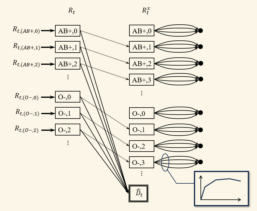
To simplify the figure, we have collapsed the network of different demand types into a single aggregate box with demand $\Dhat_t$. This network would actually look just like the network in Figure 13.1a. The decision to hold blood has to consider the value of a type of blood (including its age) in the future, which we are approximating using separable, piecewise linear value functions.
Here, we use a standard modeling trick that converts the separable, piecewise linear value function approximations into a series of parallel links from each node representing an element of $R^x_t$ into a supersink. Piecewise linear functions are not only easy to solve (we just need access to a linear programming solver), they are easy to estimate. In addition, for many problem classes (but not all) they have been found to produce very fast convergence with high quality solutions.
With this decision function, we are going to use a method called approximate value iteration where we simulate forward iteratively through time periods $t=0, \ldots, T$. Let $n = 1, \ldots, N$ be the iteration counter, where we follow a sample path of the exogenous information $W^n_t,~t=0, \ldots, T$ (these might be pulled from history, or sampled from a distribution). At time $t$, iteration $n$, we use equation $\eqref{eq:adpblood}$ to make a decision $x^n_t$ when we are in state $S^n_t$. We then observe $W^n_{t+1}$ and use our transition function (equations $\eqref{eq:bloodresourcetransition1}$–$\eqref{eq:bloodresourcetransition2}$) for the transition for $R^n_t$ to $R^n_{t+1}$. When in state $S^n_t = (R^n_t, \Dhat^n_t)$, we use our VFA policy in equation $\eqref{eq:adpblood}$ to compute $x^n_t$, and then we compute $\vhat^n_t$ to update the slopes $\vbar^{x,n}_{t-1}$. We then observe $W^n_{t+1}$ (which contains $\Dhat^n_{t+1}$) to transition to state $S^n_{t+1}$.
For most operational applications, this problem would be solved over a finite horizon (say, 10 weeks) giving us a recommendation of what to do right now. We can use the value function approximations $\Vbar^x_t(R^x_t)$ to simulate the policy a number of times, which can be used to produce a form of probabilistic forecast of future inventories.
Extensions
This is a rich and complex resource allocation problem which can be extended in a number of ways. Below are a few examples.
1) We assume that any demands that are not satisfied at time $t$ are lost. Imagine that we have emergency surgeries that have to be satisfied, and elective surgeries that can be delayed to a later time period. Write out the state variable for the new problem.
2) Assume that elective surgeries can be delayed. Consider using a value function approximation that is piecewise linear and separable in the blood inventories (this is the VFA suggested above), along with piecewise linear and separable VFAs for the amount of held demand (by blood type). We use the dual variables for the blood inventory to update the VFA for blood supplies. How might we update the VFA for the held demand?
3) Include the presence of blood that has been frozen, and the decision to freeze blood, where frozen blood that is not used has to be discarded. This means that we have to recognize that the amount of blood needed for a surgery is unknown before the surgery, when the decision to thaw the blood has to be made.
4) A hospital might require weekly deliveries of blood from a community blood bank to make up for systematic shortages. Imagine that a fixed quantity (e.g., 100 units) of blood arrives each week, but the amount of blood of each type and age (the blood may have already been held in inventory for several weeks) might be random.
5) We presented a model that focused only on blood inventories at a single hospital. We can handle multiple hospitals and distribution centers by simply adding a location attribute, and providing for a decision to move blood (at a cost) from one location to another.
This model can also be applied to any multiproduct inventory problem where there are different types of product and different types of demands, as long as we have the ability to choose which type of product is assigned to each type of demand. We also assume that products are not reusable; once the product is assigned to a demand, it is lost from the system.
What did we learn?
- We introduce a multidimensional resource allocation problem that has an extremely large state space, but offers the structure of concavity that we can exploit in the approximation of value functions.
- We show how to model a multiattribute resource allocation problem, which makes it quite easy to introduce additional attributes.
- We illustrate a basic myopic policy where the downstream impact of decisions made now is ignored.
- We then describe a VFA policy where we exploit the natural concavity of the problem to suggest an approximation based on separable, piecewise linear value function approximations.
- Our VFA policy would have to be implemented on a rolling basis, so our policy is actually a stochastic DLA, using a VFA policy for the lookahead policy. This parallels our use of dynamic programming to solve the deterministic shortest path problem which represented an approximation of our stochastic, dynamic shortest path problem in Chapter 6.
Exercises
Review questions
- What is the dimensionality of the state variable $S_t$?
- What is the dimensionality of the decision vector $x_t$?
- What are the source(s) of uncertainty?
- Describe the nature of the costs in the objective function. Where do these come from?
- What is the limitation of a purely myopic policy? What behavior would you be looking for from a better policy?
- How does the use of value functions improve the solution?
Problem solving questions
Blood management - Part I: Modeling - We are going to consider the blood management problem, but we are going to assume there is only one type of blood, although we are still going to model the aging process, where blood can be 0 to 5 weeks old. Any 5-week old blood that is held must be discarded. As in the book, there are two types of patients: urgent and elective. Let:
$R_{t\tau}$ Number of units of blood on hand at time $t$ that has been held for $\tau$ time periods, $\tau = 0, \ldots, 5$. $\Rhat_t$ New blood donations that arrive between $t-1$ and $t$, where $\Rhat_t$ is a scalar. $\Dhat^{urgent}_t$ New urgent demands that arrive at time $t$. $\Dhat^{elective}_t$ New elective demands that arrive at time $t$. At time $t$, we have to decide:
$x^{urgent}_t$ Amount of blood to be assigned to urgent patients. $x^{elective}_t$ Amount of blood to be assigned to elective patients. $x^{hold}_t$ Amount of blood to be held. $x_t$ $(x^{urgent}_t,x^{elective}_t,x^{hold}_t)$. Demands do not have to be covered, although the real issue is whether to cover an elective demand now (assuming there is enough blood to cover all the urgent demands) or hold the blood for a potential urgent demand in the future. As before, assume that any demands that are not served leave the system.
Your goal is to maximize a utility function that gives credit of 10 for each urgent patient covered and 5 for each elective patient covered.
- What is the state variable for this problem?
- What are the decision variables and exogenous information?
- What is the transition function?
- What is the objective function? Assume that we can simulate the policy in a simulator.
- Create a parameterized cost function approximation that assigns the following costs to each decision: $c^{urgent}$, penalty for not covering an urgent patient; $c^{elective}$, penalty for not covering an elective patient; and $c^{discard}$, penalty for discarding blood that exceeds the age of 5 weeks. As your policy, assume that you are going to minimize these costs at each time period. Treat the vector $c=(c^{urgent},c^{elective},c^{discard})$ as a set of tunable parameters. Describe how to optimize the vector $c$ using a stochastic gradient algorithm. Be sure to give the equation for calculating the stochastic gradient.
- Blood management - Part II: Backward approximate dynamic programming - We are now going to design a policy based on the idea of approximating the value function using backward approximate dynamic programming. This means that you have to specify a linear model to approximate $V^x_t(S^x_t)$. The details of this model are not that important, but you might use something like
$$
\Vbar^x_t(S^x_t) = \thetabar_{t0} + \sum_{age=0}^5 \theta_{t1,age} R^{urgent,x}_{t,age} + \sum_{age=0}^5 \theta_{t2,age} R^{elective,x}_{t,age}.
$$
For the purposes of this exercise, you can just write $\Vbar^x_t(S^x_t) = (\theta_t)^T \phi(S^x_t)$ where $\theta_t$ is a column vector of coefficients and $\phi(S^x_t)$ is a column vector of features.
- Define the post-decision state, and use this to write Bellman's equation to characterize an optimal policy. You will need to write an expression for the value $V_t(S_t)$ of being in the pre-decision state $S_t$ at time $t$ in terms of the value $V^x_t(S^x_t)$ of being in post-decision state $S^x_t$. You will then need to write an expression for $V^x_t(S^x_t)$ in terms of $V_{t+1}(S_{t+1})$. Assume that units of blood are always integer.
- What is the dimensionality of the pre- and post-decision state variables? Do we care how large the state space is?
- Write out detailed pseudo-code that describes how to estimate the value function approximations for this problem over a finite horizon $0, \ldots, T$. Think of this as a programming exercise without the actual programming. It has to be detailed enough that you could hand it to a classmate in the course (and familiar with the material) who could then write the code.
- Write out the policy using your expression for the approximate value function.
- Blood management - Part III: Lookahead policy - This time, we are going to assume that we have rolling forecasts of supplies and demands. Let $f^R_{tt'}$ be the forecast of blood donations at time $t'$ made using what we know at time $t$. Let $f^{D,urgent}_{tt'}$ and $f^{D,elective}_{tt'}$ be the forecasts of new urgent and elective demands arriving at time $t'$ given what we know at time $t$. Assume that forecasts are provided exogenously (that is, we do not have to model how the forecasts evolve from $t$ to $t+1$). You may use
$$
\begin{align*}
f^R_t &= (f^R_{tt'})_{t'=t+1}^T, \\
f^{D,urgent}_t &= (f^{D,urgent}_{tt'})_{t'=t+1}^T, \\
f^{D,elective}_t &= (f^{D,elective}_{tt'})_{t'=t+1}^T, \\
f_t &= (f^R_t,f^{D,urgent}_t,f^{D,elective}_t).
\end{align*}
$$
Let $\sigma^R_{t'-t}$ be the standard deviation of the error between the actual donations $\Rhat_{tt'}$, which we assume is known based on past performance. We assume that this is purely a function of how far into the future we are planning, given by $t'-t$. Similarly let $\sigma^{D,urgent}_{t'-t}$ and $\sigma^{D,elective}_{t'-t}$ be the standard deviations of the errors in the forecasts of new urgent and elective demands.
- Model the five elements of a sequential decision problem for this setting. You should be able to copy elements from one of the previous parts to this problem. Feel free to reference any equations by number you wish to re-use. The major change is the inclusion of the forecasts.
- Write out a DLA policy using a deterministic lookahead with forecasts as point estimates of any future donations and demands.
- Now design a parameterized policy where you replace each forecast with one that is some number of standard deviations above (or below) the point forecast. Use three parameters, which you might designate $\theta = (\theta^R, \theta^{urgent}, \theta^{elective})$. Write the problem of finding the best value for $\theta$ as an optimization problem. Explain any assumptions you have to make in your formulation.
- Your objective function in part (c) involves approximating an expectation. You can do this via simulation, where you would simulate a sample path $\omega$ over a horizon of $T$ time periods. What is meant by $\omega$?
- Give the formulas for computing the mean and sample variance of the performance of a policy from $L$ simulations using sample paths $\omega^1, \ldots, \omega^L$.
- Assume that you represent the set of possible values of the vector $\theta$ by the sample $\theta^1, \ldots, \theta^K$. Describe a search method using interval estimation parameterized by $\lambda^{IE}$ (in the book we used $\theta^{IE}$, but this creates too many $\theta$'s). You will need to describe your belief model and how it is updated after each time you run a simulation using $\theta = \theta^k$. Assume you have a budget of $N$ simulations, and that $\lambda^{IE}$ is known.
Programming questions
These exercises use the Python module BloodManagement on tinyurl.com/sdagithub.
Our goal is to manage the assignment of different blood types to different patients, who are characterized first by their own blood type, and second by whether the surgery is urgent or elective.
This exercise will have you working with two classes of policies: a myopic parametric cost function approximation, and a policy based on value function approximations.
We are going to begin by assuming that you are just going to match different blood types to different demands. Blood is described by blood type (of which there are eight) and age, which will range from 0 to 2 weeks (3 week-old blood is discarded). Patients are described by blood type and whether the surgery is urgent or elective. There are various bonuses and penalties that guide assignments. For example, there are positive bonuses for covering urgent patients (this is highest). There is also a bonus for matching blood types exactly (e.g. A-positive blood with an A-positive patient), and a penalty for discarding blood after it becomes too old.
If we ignore the impact of decisions now on the future, we have a simple linear program that matches supplies and demands, with costs given by this set of bonuses. The problem is that by ignoring the impact of decisions now on the future, we may find that we are not doing the best that we can. One issue that arises is when we use blood now for elective surgery, we are ignoring that this might be useful to hold onto in case we run out of blood for urgent surgery later on. Alternatively, we may use O- blood now rather than hold it for the future when we might run out of other blood types.
Let $R_{ta}$ be the supply of blood with attribute $a$ for week $t$, and let $R_t = (R_{ta})_{a\in\Acal}$ where $\Acal$ is the set of all the different blood attributes (blood type and age). Similarly let $D_{tb}$ be the attributes of a patient where $b$ captures the blood type and whether the surgery is urgent or elective, and let $D_t = (D_{tb})_{b\in\Bcal}$. The state of our system is $S_t = (R_t,D_t)$.
Now let $\Rhat_{t+1,a}$ be the number of units of blood with attribute $a$ that were donated between weeks $t$ and $t+1$. Similarly let $\Dhat_{t+1,b}$ be the number of new patient arrivals with attribute $b$. We would write
$$ W_{t+1} = (\Rhat_{t+1,a},\Dhat_{t+1,b}). $$Finally let $\omega$ represent a sample path $W_1(\omega), \ldots, W_T(\omega)$ of donations and new patients over our $T$-week horizon. Assume that we have created a set of simulations of $W_t$, and let $\Omega=(\omega_1, \ldots, \omega_N)$ be this set of sample realizations.
- How many dimensions does the state variable $S_t$ have?
- Let $X^\pi(S_t\vert \theta)$ be the result of solving the linear program given the state $S_t$, where $\theta$ is the vector of all the bonuses and penalties for different assignments. Let $D^{urgent}_t(x_t)$ be the number of urgent patients that were covered given the decision vector $x_t$, and let $D^{elective}_t(x_t)$ be the number of elective patients that were covered. Write the problem of finding the best value of $\theta$ as an optimization problem, where instead of our usual expectation you are going to write it as an average over the sample paths in $\Omega$.
- We are going to consider a dataset where there is a probability that demand occasionally surges. You can set this probability in the spreadsheet. Set this surge probability to 50 percent. There is a special penalty for using blood to cover elective surgery to encourage the myopic model to save blood for urgent surgery that might have an increase in demand later on. Find the best value of this penalty in the set $\lbrace -4,-9,-14,-19,-24\rbrace $ after running 20 testing iterations.
- Without doing any additional numerical work, imagine now that the penalty on the O-negative blood needs to depend on the week to handle seasonal variations. Since you are simulating 15 weeks, describe a method for optimizing over a 15-dimensional vector (we have described two core strategies in prior assignments - you may pick one, or invent a new one).
Now we are going to switch to a VFA-based policy, where we use the marginal value of each blood type (and age) that is held for the future. This will be done with an adaptive learning algorithm that was described in the VFA policy section above (and very similar to our ADP strategy for the shortest path problem, except now we are doing it for a problem where the decision is a vector).
Set the penalty for using blood on electives to 0. When using a VFA-based policy, the VFA should learn that urgent blood in excess of supply might be needed in the future. When you are using the VFA policy, you will need to run 20 training iterations to estimate the value functions. After these are estimated, you will then run 20 testing iterations to evaluate the quality of the policy.
We are going to test our policies for a dataset where there is a probability demand occasionally surges. You can set this probability in the spreadsheet. Begin by setting this surge probability to 0.7.
- The adaptive learning algorithm requires estimating the marginal value of each blood type. Let $\vhat^n_{ta}$ be our estimate of the marginal value of blood type $a$ for week $t$ while simulating sample path $\omega^n$. Let $\Vbar^{n-1}_t(R_{ta})$ be our estimate, after $n-1$ iterations, of the marginal value of the $r$th unit of blood where $r = R^x_{ta}$ at the end of week $t$ (this is our "post-decision" state variable). Recall that we use $\vhat^n_{ta}$ to update the value function approximation around the previous post-decision state variable. We write this updating process as $$ \Vbar^n_{t-1,a}(R^{x,n}_{t-1,a}) = (1-\alpha) \Vbar^{n-1}_{t-1,a}(R^{x,n}_{t-1,a}) + \alpha \vhat^n_{ta}. $$ Our first task is that we have to tune $\alpha$. Run the approximate dynamic programming algorithm for 20 iterations (this is how the spreadsheet is set up) for $\alpha \in \lbrace 0, 0.05, 0.1, 0.2, 0.3\rbrace $ and report the results. Note that a stepsize $\alpha = 0$ is the same as keeping the value function approximation equal to zero (in other words, the myopic policy). If $\alpha = 0$, you do not have to train the VFAs, so you just have to run the 20 testing iterations to evaluate the policy. How well does the VFA policy perform relative to the myopic policy (corresponding to $\alpha = 0$)?
- Now switch the surge probability to zero, and compare the myopic policy to the VFA policy using a stepsize of $\alpha = 0.2$. How do these compare? Can you explain the behavior for this dataset compared to when there were surges?