Chapter 7: Applications, revisited

Now that we have reviewed a series of problem settings, we are going to pause and use these applications to illustrate in greater depth some of the modeling issues we touch on in Chapter 1.

Starting with the inventory problems in Chapter 1, we have now covered six classes of sequential decision problems. For each problem, we illustrated one or two strategies for making decisions:

• Chapter 1) Inventory problems – We introduced sequential decision problems using variations of a simple inventory problem. Policies included order-up-to, and a policy based on adjusted forecasts.
• Chapter 2) Selling an asset – We had to decide when to sell a financial asset. Policies included variations of buy-low, sell-high.
• Chapter 3) Adaptive market planning – This problem used a derivative-based stochastic search, where the sequential decision problem was choosing a stepsize, which we illustrated using simple parametric functions.
• Chapter 4) Learning the best diabetes treatment – This is a classic active learning problem known as the multiarmed bandit problem. We designed policies based on parameterized optimization problems.
• Chapter 5) Static stochastic shortest paths – We found an optimal solution of a particular version of a stochastic shortest path problem using a classical dynamic programming recursion that we could solve exactly, and then introduced a more complex stochastic version that we solved using approximate dynamic programming, exploiting a post-decision state variable.
• Chapter 6) Dynamic stochastic shortest paths – Here we switch to a dynamic shortest path problem where estimates of the expected path costs evolve over time (in the static case in Chapter 5, our estimates of the expected costs did not change). We used this to illustrate a basic deterministic lookahead policy, and a parameterized lookahead policy.

Earlier, we introduced four classes of policies. In the applications we have reviewed so far, we have seen illustrations of each of the four classes. In this chapter, we are going to review the four classes in greater depth, and then we will return to our set of applications and identify the class for each of the suggested policies.

The four classes of policies

We first observe that the four classes of policies can be divided into two categories: the policy search class, and the lookahead class. Each of these can then be further divided into two classes, creating the four classes of policies. These are described in more detail below.

Policy search

The “policy search” class of policies involves searching over a set of functions for making decisions to find the function that works the best on average, using whatever objective is appropriate for the problem. Most of the time this will mean searching for the best value of a set of parameters that characterize a parameterized policy, but it also means that we may have to evaluate different parameterizations.

Policy-search policies can be divided between two classes:

• Policy function approximations (PFAs) – These are analytical functions that directly map a state to an action. Some examples are:
  • A parameterized function such as the “high-low” policy given in Chapter 2, which we repeat here
  \[X^{high-low}(S_t\vert \theta^{high-low}) = \begin{cases} 1 & \text{if } p_t < \theta^{low} \text{ or } p_t > \theta^{high}, \\ 1 & \text{if } t=T, \\ 0 & \text{otherwise.}\end{cases}\]

  where $\theta^{sell-low} = (\theta^{low},\theta^{high})$. Other examples are the order-up-to policy we saw in Chapter 1, and the adjusted forecast policy.

  • A linear function, such as
  \[X^\pi(S_t\vert \theta) = \theta_0 + \theta_1 \phi_1(S_t) + \theta_1 \phi_1(S_t) + \ldots + \theta_F \phi_F(S_t)\]

  where $(\phi_f(S_t)),~f=1, \ldots, F$ is a set of features (“linear” means linear in the parameter vector $\theta$ – the features $\phi_f(S_t)$ can be highly nonlinear in $S_t$). For example, we might be trying to decide how much to bid to have a movie advertised on a website, and a feature might be the genre of the movie or the name of the lead actor or actress.

  Linear functions (also known as “affine policies”) are popular, but note that you could not use a linear function to approximate step functions such as the buy-low, sell-high or order-up-to policies illustrated above.

  • Advanced functions such as locally linear functions or neural networks, although these typically have large numbers of parameters (the weights in a neural network) that need to be tuned.
• Cost function approximations (CFAs) – These are policies that require solving a parameterized optimization problem, where we may parameterize either the objective function or the constraints. CFAs open the door to solving high-dimensional decision problems. Some examples are:
  • A simple example of a parameterized cost function approximation is the interval estimation policy we introduced in Chapter 4 and repeat here
  \[X^{IE}(S^n\vert \theta^{IE}) = \argmax_{x\in\Xcal} \left(\mubar^n_x + \theta^{IE} \sigmabar^n_x \right).\]
  • Parameterized optimization models – We saw this in Chapter 6 when we chose the $\theta$-percentile of the link costs. This is a widely used heuristic in industry that has been overlooked by the research literature. Airlines use this idea to optimize the movement of their aircraft and crews in the presence of significant weather delays. Grid operators planning the scheduling of energy generators will insert reserve capacity to make sure that demand can be covered if a generator fails.

Both PFAs and CFAs have parameters that have to be tuned. The only difference is whether the policy involves an embedded optimization problem or not. Both are exceptionally powerful and are widely used in different settings.

Lookahead approximations

Policies based on lookahead approximations are constructed by approximating the downstream costs (or rewards) from making a decision now, which are then considered along with the initial cost (or reward) of the initial decision.

• Policies based on value function approximations (VFAs) – These are policies that are based on Bellman’s equation. The most basic form of Bellman’s equation for deterministic problems was first presented in Chapter 5 as

There are many problems where the transition to $S_{t+1}$ involves information (contained in $W_{t+1}$) that is not known at time $t$, which means $S_{t+1}$ is a random variable at time $t$. In this case, we have to insert an expectation as we did earlier which gives us

In practice, we typically have to replace the value function $V_{t+1}(S_{t+1})$ with an approximation $\Vbar_{t+1}(S_{t+1})$, as we did in the approximate dynamic programming section of Chapter 5. The field that studies these approximations goes under names such as approximate dynamic programming, reinforcement learning (which originated in computer science), and adaptive dynamic programming (the term used in the engineering controls community). In this case, the policy would be given by

If we use the post-decision state $S^x_t$, we can write our policy as

which we illustrated in Chapter 5.

We used the deterministic shortest path problem to illustrate an application where value functions could be computed exactly. This can sometimes be done in stochastic problems, but in most applications, it has to be done approximately. The challenge is doing computations that are of sufficiently high quality to produce effective policies.

A popular approximation strategy for value functions is to use a linear model given by

where $(\phi_f(S^x_t))_{f\in\Fcal}$ is a user-defined set of features and $\theta^{VFA}$ is a set of parameters chosen using approximate dynamic programming algorithms.

We fit the linear model by collecting “observations” of the value $\vhat^n_t$ of being in state $S^n_t$ in the $n$th iteration. Let $\thetabar^{VFA,n-1}$ be the estimate of $\theta^{VFA}$ after $n-1$ updates. There are methods that allow us to use $\vhat^n_t$ to easily update $\thetabar^{VFA,n-1}$ and obtain $\thetabar^{VFA,n}$. This gives us a VFA policy that we can write as

Approximating value functions using linear models has been very popular, but there are virtually no theoretical guarantees on the quality of the resulting solution. Even worse, there is empirical evidence that the results can be quite poor. Yet, it remains popular because it is an easy way to “get a number.”

Also popular today is to use neural networks (especially deep neural networks) to approximate a value function. Neural networks are attractive since they avoid the need to design the set of features $(\phi_f(S_t))$ for $f\in\Fcal$. Caution has to be used, especially when we have to work with noisy observations of the value function, since the massive flexibility of neural networks can cause overfitting.

• Direct lookahead approximations (DLAs) – The first three classes of policies require finding some form of a functional approximation: the policy (for PFAs), the function being optimized (for CFAs), or the value of being in a downstream state (for VFAs). However, there are many problems where these functional approximations are just not possible.

  The “right” way to solve a DLA is to solve the true problem in the future, starting from the state $S_{t+1}$ produced by starting in state $S_t$, taking action $x_t$, and then observing the random information $W_{t+1}$. The hard part is that in addition to modeling future uncertainties $W_{t+1}, W_{t+2}, \ldots$, we also have to make optimal decisions $x_{t+1}, x_{t+2}, \ldots$, each of which depend on the future state $S_{t+1}, S_{t+2}, \ldots$, which are random.

  Although it is quite messy (and perhaps frightening), this policy means solving

If we could compute equation $\eqref{eq:policiesDLA}$, we would have an optimal policy. It is quite rare that equation $\eqref{eq:policiesDLA}$ can be solved exactly. The basic stochastic shortest path problem in Chapter 5 is an example, but this is because uncertainty arises in a particularly simple way.

In most applications, we approach solving $\eqref{eq:policiesDLA}$ by solving an approximate lookahead model. Instead of writing our sequence of states, decisions and information as

we create a simplified set of states, decisions and information for a model that we are solving at time $t$ that we represent using

where $\Stilde_{tt’}$ is typically a simplified state variable for the lookahead model we create when making a decision at time $t$, for time $t’$ in the lookahead model. $\xtilde_{tt’}$ is our (possibly simplified) decision created for time $t’$ in the lookahead model, and $\Wtilde_{tt’}$ is the simplified information process at time $t’$ in the lookahead model. Decisions $\xtilde_{tt’}$ are made using a lookahead policy $\Xtilde^{\tilde \pi}t(\Stilde{tt’})$ which is typically a simplified policy chosen because it is easy to compute.

Our policy based on our approximate lookahead model would be written as

Equation $\eqref{eq:policiesapproximateDLA}$ is illustrated using the decision tree in Figure 7.1, which illustrates the use of approximate states, decisions and uncertainties as we look into the future. Creating these approximations requires a blending of art and science. We want to strike a balance between accurately modeling the future while balancing computational requirements.

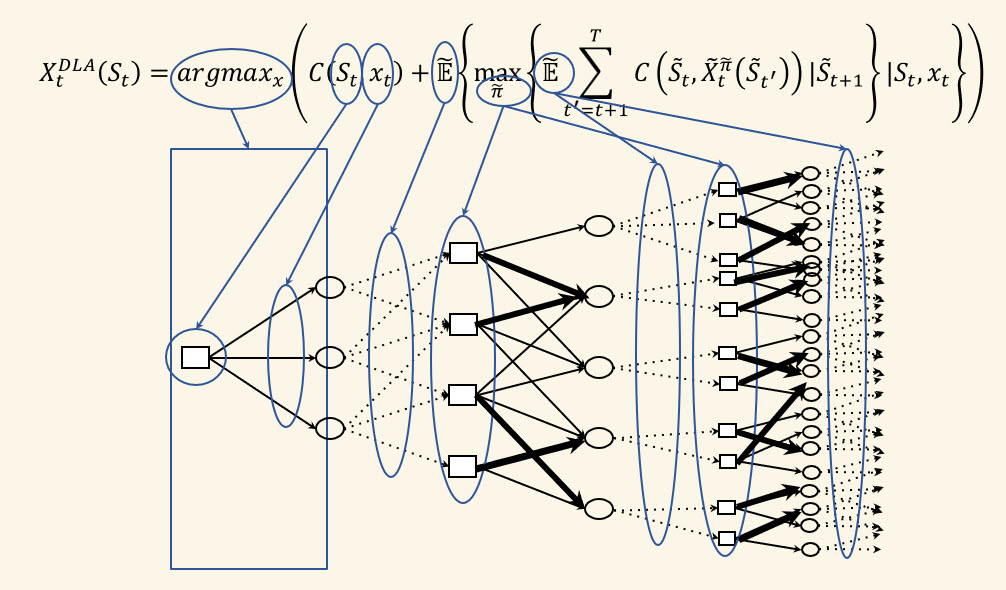
The design of the lookahead policy $\tilde \pi$ (sometimes called the policy-within-a-policy) is highly problem dependent. In fact, we can use any of our four classes of policies. The key is that it has to be computationally simple, since we will have to compute it many times. Remember that the lookahead model does not have to be exact (in most cases we could never solve it if we tried to use an exact lookahead model). Instead, we are choosing approximations that we think will produce good decisions now, by approximating decisions that we might make in the future.

We have already seen applications of this approach. For the dynamic shortest path problem in Chapter 6, we turned to the widely used approach of solving a deterministic lookahead model, where we take the best estimate of what might happen in the future and solve a deterministic optimization problem. This approach ignores the effect of future uncertainties, but we introduced the idea of using a parameterized deterministic optimization problem. However, we have to tune the parameter.

These four classes of policies (PFAs, CFAs, VFAs and DLAs) are universal, which is to say, any policy chosen for a sequential decision problem (any sequential decision problem) will be one of these four classes. However, these can also be building blocks for hybrid policies.

We have illustrated all four classes of policies, which leaves the question: How do you know which one to use? Sometimes it will seem obvious, such as finding the best path to a destination. For problems like this, a direct lookahead is a natural choice. But there are problems where any of the four classes is a viable candidate.

Two problems where we have successfully demonstrated all four classes are the inventory problems in Chapter 1, and the diabetes learning problem in Chapter 4. The key is to think carefully about all four classes of policies, rather than just focusing on one, which is what is happening so often today.

Models, revisited

In this section we are going to do a tour through the different applications, starting first with a review of the state variables. Then we are going to review the different policies, and classify the policies we have seen into the four classes.

State variables, revisited

There is considerable confusion in the academic literature about what is meant by a state variable, as evidenced by the noticeable absence of definitions of what a state variable is in books on dynamic programming, stochastic programming, and reinforcement learning.

The only exception to this pattern, which really stands out, is the optimal control literature where definitions of state variables are quite common. In the controls community, a state variable is commonly defined as “all the information we need at time $t$ to model a system from time $t$ onward.” What is missing, however, is any description of precisely what information is needed to model the system from time $t$ onward.

We define two versions of state variables (from Reinforcement Learning and Stochastic Optimization, Section 9.4):

A state variable is:

a) Policy-dependent version – A function of history that, combined with the exogenous information (and a policy), is necessary and sufficient to compute the cost/contribution function, the decision function (the policy), and any information required by the transition function to model the information needed for the cost/contribution and decision functions.

b) Optimization version – A function of history that is necessary and sufficient to compute the cost/contribution function, the constraints, and any information required by the transition function to model the information needed for the cost/contribution function and the constraints.

We need the two versions since if we have a system where we have specified the structure of a policy, we need to be sure we include any information needed by the policy. For example, we may have an inventory problem, where we consider two policies: one that uses a forecast of future demands, while the other just uses an order-up-to policy. While a forecast certainly seems relevant, if we are using an order-up-to policy, we are not using the forecast, and as a result it would not be in the state variable.

It helps to do a tour through our applications up to now and review the state variables for each one. For each application, we are going to summarize the state variable, which we might write as $S_t$ or $S^n$ depending on the setting, and we are going to classify the elements as physical state variables $R_t$, informational variables $I_t$, and belief state variables $B_t$.

Chapter 1 – This chapter introduced two inventory problems that were also designed to bring out different flavors of state variables. The simple inventory problem was characterized by a state variable $S_t$ that consists of just the inventory $R^{inv}_t$ at time $t$. This problem is one of the most widely used applications for illustrating dynamic programming.

The more complex inventory problem required a state variable

This state variable illustrates all three classes of information in state variables: the physical state variables $R_t = R^{inv}t$, other information $I_t = c_t$, and belief state variables $B_t = (f^D{t,t+1}, \sigmabar^D_t, \sigmabar^f_t)$ where $(f^D_{t,t+1},\sigmabar^D_t,\sigmabar^f_t)$ captures the forecasted mean and standard deviation of the error of the future demand $\Dhat_{t+1}$, and the standard deviation in the change in forecasts from time $t$ to $t+1$ (we assume that the change in forecasts have mean zero).

Chapter 2 – This chapter introduced a simple asset selling problem with state variable

where the physical state variable $R_t$ captures whether we are still holding the asset or not (it could have also held how many shares of stock we were holding), and the informational state $I_t = p_t$ is the price at which we sell the stock.

We also introduced the idea of computing a smoothed estimate of the price of the asset using

We then designed a policy that made decisions based on how much the price $p_t$ deviated from this smoothed estimate. Now our state variable becomes

Now imagine that when we decide to sell our stock at time $t$, we sell at an unknown price $p_{t+1}$ which evolves according to

where $\varepsilon_{t+1}$ is a mean 0 noise term. Now our state variable would look like

Chapter 3 – Here we described a gradient-based search algorithm that evolves according to a classical stochastic search iteration given by

This procedure is a method for searching for the best value of $x$, but this is a sequential decision problem where the stepsize $\alpha_n$ is the decision. If we choose the stepsize with a deterministic formula such as $\alpha_n =1/n$, then the “state” of our search procedure is

However, we might use an adaptive (stochastic) stepsize formula such as

where $N^n$ is the number of times the gradient $\nabla_x F(x^n,W^{n+1})$ changes direction, then we need to know $N^n$, and our state variable becomes

Chapter 4 – Our diabetes problem is an instance of a pure learning problem, where we are trying to learn the true response $\mu_x$ of a patient to a drug. After trying several drugs, we might capture our belief using the state

where we assume that the true response $\mu_x \sim N(\mubar^n_x, (\sigmabar^n_x)^2)$.

This belief model might work if we have a different belief for each patient, but presumably we start with a body of knowledge of how the drug works across all patients. We might capture this in an initial state

Now imagine that the $n$th patient arrives with attributes $a^n$ (gender, weight, smoking history, …). The response of the patient to drug $x$ would depend on both the drug as well as the attributes of the patient. This means that our state variable (that is, the information we have available to make the decision) consists of information we do not control (the attributes of the patient $a^n$), and information we do control (the choice of drug $x^n$). So we would write our state variable (the information we use to make the decision) as

where we decided to put $a^n$ in our informational state variable $I^n$, and the variables $(\mubar^n_x, \sigmabar^n_x)$ in the belief state variable $B^n$.

Chapter 5 – For our stochastic shortest path problem, we started with a basic problem where a traveler incurs a random cost when traversing a link, but only knows the mean and variance of the costs before making a decision at node $i$ which link $(i,j)$ to traverse. For this problem, the state of our traveler is simply the node $N_t$ where he is located after traversing $t$ links, giving us

We then transitioned to a problem where the traveler at node $i$ gets to see the actual costs $\chat_{tij}$ that would be incurred if he were to travel over the link $(i,j)$. With this additional information, the state variable becomes

Chapter 6 – We considered a dynamic shortest path problem where the estimated cost on link $(i,j)$, $\cbar_{tij}$, evolves over time. That is, at time $t+1$, we assume we are given an updated set of estimates that we would denote $\cbar_{t+1}$. Imagine that our traveler is at node $N_t= i$. The state of our system (for our traveler) would then be given by

Now imagine that we show the traveler a path that we designate $p_t$ which is the set of links that we are planning to get from his current node $N_t$ to the destination. Let’s say that we just updated the path, and have asked the traveler if he accepts the new path. If he says yes, the navigation system will continue to re-optimize, but will introduce a small bonus for staying with the latest path $p_t$ that the traveler just accepted (this is done to prevent the system from chattering between two nearly equivalent paths).

If $p_t$ is the most recently accepted path, then this is information that we need to make decisions in the future. In this case, our state variable becomes

These decision problems have illustrated all three types of state variables: physical state variables $R_t$, informational state variables $I_t$, and belief state variables $B_t$. We have seen problems that have just $R_t$, or just $B_t$, and combinations with $I_t$ such as $(R_t, I_t)$ and $(I_t, B_t)$, as well as all three $(R_t, I_t, B_t)$. We emphasize that the distinction between $R_t$ and $I_t$ can sometimes be arbitrary, but there are so many problems that involve managing physical or financial resources (buying, selling, moving, modifying), with decisions that affect (or are constrained by) physical or financial resources, that we felt it was necessary to create a special class just for resources.

We think that there are many problems involving uncertainty that also involve learning, and may involve active learning since decisions may impact what we observe (as in the diabetes example). We suspect that as modelers become comfortable with including belief state variables in sequential decision problems that we will see them used more often.

Policies, revisited

Our six application settings (and in some cases the extensions) were chosen to expose each of the four classes of policies. Below we review the different policies and identify the class to which they belong.

Chapter 1 – We introduced two inventory problems. One used an order-up-to policy of the form

while the second used a policy of bringing the inventory up to the forecasted demand plus a buffer

Both of these policies involve one or two tunable parameters. Both are analytical functions that do not have an embedded optimization operator ($\min$ or $\max$). These are the distinguishing characteristics of a policy function approximation (PFA).

Chapter 2 – This chapter addressed the problem of determining when to sell an asset. Several policies were suggested, but representative samples are the “sell-low” policy given by

and the “tracking policy”

Both of these policies are similar to our “order-up-to” inventory ordering policy in that they are parametric functions with tunable parameters, which means they are additional examples of policy function approximation (PFA). While this is hardly the only way to solve an asset selling problem, this class of policy is fairly popular on Wall St.

PFAs are popular in practice because of their simplicity and transparency, but it is important to keep in mind: The price of simplicity is tunable parameters… and tuning is hard!

Chapter 3 – Adaptive market planning – This problem involves using a popular gradient-based search method (see equation $\eqref{eq:stochasticgradientaltransitionrevisited}$) where the stepsize $\alpha_n$ is the decision. If we had a deterministic problem, we would compute $\alpha_n$ by solving the one-dimensional optimization problem

which is a form of direct lookahead approximation (DLA). However, when we have to deal with uncertainty, a one-dimensional search means we have to be able to compute the expectation $F(x) = \E F(x,W)$ which is generally not possible in practice. Instead, we might use a deterministic policy such as

where we have written this as a parameterized function (that is, a form of PFA). We also illustrated an adaptive (state-dependent) policy given by equation $\eqref{eq:adaptivealpharevisited}$ where we replaced $n$ with a counter $N^n$ that counts how many times the gradient changes direction (or we could count how many times the objective function does not improve). We would write this policy as

where our state $S^n$ carries the information $N^n$.

Side note: PFA-style policies are universally used in stochastic gradient algorithms. While these may in fact be best, the reality is that no one has even tried using the other three classes of policies. Might be worth a look.

Chapter 4 – Learning the best diabetes treatment – This is a pure learning problem which we have approached using the highly popular class of policies known as upper confidence bounding. Perhaps the best known UCB policy is given by

Another variant which works very well was originally introduced as interval estimation which is given by

Finally, a variant that was originally discovered in 1933 and then re-discovered a few years ago is Thompson sampling, which is given by

where $\muhat^n_x$ is randomly sampled from a normal distribution with mean $\mubar^n_x$ and variance $\theta^{TS} \sigmabar^n_x$.

Note that all three policies share two features: an optimization operator (an $\argmax_x$ for these policies) and a tunable parameter. These can be viewed as parameterized optimization problems, which belong to the class parametric cost function approximation (or CFA).

CFA policies are widely used in practice, but have received very little attention in the academic literature outside of the specific application of learning policies such as our diabetes application. We are going to see this idea applied in a very different setting in later chapters.

Chapter 5 – Static stochastic shortest paths – Our first stochastic shortest path problem assumed that a traveler incurred stochastic costs, but these were learned only after traversing a link. This assumption allowed us to solve the problem as a deterministic shortest path problem, which is easily solved using Bellman’s equation, giving us a policy that is given by

where $S_t = N_t = i$ is the node where the traveler is located. The value functions $V_t(S_t)$ are computed by working backward in time, starting at $t=T$ where we set $V_T(S_T) = 0$ for all nodes $S_T$. This is a form of policy based on value function approximations, and this is a rare case where a VFA policy is actually optimal.

We then transitioned to a harder problem where a traveler is allowed to see the costs $\chat_{tij}$ out of node $i = N_t$. For this problem, the state variable becomes $S_t = (N_t, (\chat_{t,N_t,j},~j\in\Ncal^+_i))$. For this problem we had to approximate the value function using the post-decision state $S^x_t = N^x_t$ where $N^x_t$ is the node we have chosen to go to after making our decision $x_t$ when we are at node $N_t$. In this case our policy looked like

This again is a VFA-based policy, but this time it is no longer optimal since $\Vbar^x_t(S^x_t)$ is an approximation we had to estimate from data. With some care, however, we can devise an asymptotically optimal policy.

Chapter 6 – Dynamic stochastic shortest paths – This is where we encounter a problem where the estimated cost on each link $\cbar_{tij}$ is evolving over time. So, at time $t$, $\cbar_t$ is the vector of estimated link costs, that becomes $\cbar_{t+1}$ the next time period. This means that our state variable transitions from $S_t = N_t$ which is just the node where the traveler is located, to $S_t = (N_t, \cbar_t)$ which is an extremely high-dimensional state variable. This is not a problem we can approach even with approximate dynamic programming (it is hard to envision a VFA built around this state variable).

Instead, we propose the idea of using a lookahead model, where we ignore the fact that as the traveler progresses over the network the vector of estimated link costs $\cbar_t$ will evolve over time. Instead, we can assume it is fixed (and let’s assume deterministic). This means we now have a lookahead model that is, in fact, a deterministic shortest path problem, but we have to remember that we are optimizing a deterministic lookahead model, which is a DLA policy. Of course, we know how to do this optimally, but an optimal solution to an approximate lookahead model is not an optimal policy!

Deterministic lookaheads are popular, but there is a way to make them even better, without making them more complicated. We introduced that idea when we suggested using the $\theta$-percentile of the cost rather than the mean $\cbar_t$. Let $\ctilde_{tij}(\theta)$ be the $\theta$-percentile of the cost on link $(i,j)$ given what we know at time $t$. Now, solve a deterministic lookahead model using the costs $\ctilde_{tij}(\theta)$. Now we have a parameterized deterministic lookahead model, which is a hybrid of a parametric CFA and a DLA.

Online vs. offline objectives

There are two perspectives for evaluating the performance of a policy:

• Online learning – There are many settings where we have to learn as we go in the field. For example, we might be trying to learn the best price for a product, the best path through a congested city, or the best drug for a patient to lower blood pressure. In each of these cases, we want to do as well as we can given what we know, but we are still learning so we can make better decisions in the future. This means we need to maximize the cumulative reward over time (or iterations) so we capture how well we are doing while we are learning.
• Offline learning – In other cases, we can learn in a laboratory setting, which might be a physical lab (to test different materials or observe the performance of a drug on mice), a computer simulator, or even a field setting which is being run as a test market (to evaluate a product) or a clinical trial (to test drugs). If we are learning in a laboratory environment (“offline”) then we are willing to perform trial and error without worrying about how well we do. Instead all we care about is the quality of the solution in the end, which means we want to optimize the final reward.

A word of caution about the terms online and offline. In the machine learning community, “offline” refers to the estimation of models using a single, batch dataset. By contrast, online learning is used to refer to fully sequential settings where data arrives over time. This is typically in field situations where data is created by some exogenous process (such as observing patients arriving to a doctor’s office), which is the same setting we assume when using the term “online.” However, in machine learning “online” would still be used to refer to an iterative algorithm being used in a simulation.

There are entire fields dealing with sequential decision problems that are separated by whether they focus on final reward or cumulative reward. For example, communities that work on “stochastic search” tend to focus on final reward, while the communities that work on “multiarmed bandit problems” (a form of stochastic search problem) generally optimize cumulative reward. The reality is that you can use the same policy for either objective, but you have to tune it for the objective you choose.

Online (cumulative reward) optimization

It is typically the case when doing policy search that we have a parameterized policy that we can write as $X^\pi(S_t\vert \theta)$. The decision $x_t = X^\pi(S_t\vert \theta)$ might be the price of a product, the choice of a blood-pressure drug or the bid placed to maximize ad-clicks. In all these cases, we have to learn as we go, which means we need to maximize performance as we are learning.

Let $C(S_t,x_t)$ be our performance metric (revenue, reduction in blood-pressure, or net revenue from ad-clicks). We want to find $\theta$ that produces the policy $X^\pi(S_t\vert \theta)$ that solves the optimization problem

where $S_{t+1} = S^M(S_t, X^\pi(S_t\vert \theta),W_{t+1})$. The expectation in $\eqref{eq:derivativebasedonline}$ is over all possible realizations of $W_1, \ldots, W_T$, as well as over the possible values of uncertain parameters (such as uncertain initial beliefs about market responses or how someone responds to a drug) that are contained in the initial state $S_0$.

Equation $\eqref{eq:derivativebasedonline}$ is an example of an “online” or “cumulative reward” objective function, since we want to maximize the sum of all the rewards over some horizon. This is of particular interest in online learning problems where we have to learn the performance, such as revenue from a price or the performance of a drug for a particular patient, which means balancing the process of learning while also trying to do as well as we can.

Offline (final reward) optimization

In offline settings, we typically have a budget of $N$ experiments. A classical (if inappropriate) problem that is often used to illustrate offline, derivative-free learning is the newsvendor problem which we addressed in Chapter 3. As a reminder, the newsvendor problem is written as

where $x$ is the quantity of resource we order at a unit cost $c$, which is then used to meet the demand $W$ (which is unknown when we choose $x$). We assume the distribution of $W$ is unknown.

Let $x^n = X^\pi(S^n\vert \theta)$ be our choice of $x$ given what we know which is captured by $S^n$, where our policy $X^\pi(S^n\vert \theta)$ depends on one or more parameters in $\theta$. After we implement $x^n$, we observe $W^{n+1}$, update $S^{n+1}$ and then repeat the process. After $N$ iterations, we obtain a final design we denote $x^{\pi,N}(\theta)$.

We now have to evaluate our final design $x^{\pi,N}(\theta)$. To perform this evaluation, we have to consider two, and possibly three, sources of uncertainty. The first is that we may have uncertainty in unknown parameters such as the mean of $W$. For example, $W$ might come from a Poisson distribution with mean $\mu$, and we may assume that $\mu \in {\mu_1, \ldots, \mu_K}$ where $p_k = Prob[\mu = \mu_k]$. The distribution $(p_k)_{k=1}^K$ is contained in the initial state $S_0$.

Then we have the random arrivals of demands $W^1, \ldots, W^N$ which would be sampled from a distribution with mean $\mu$. We use these observations, and the policy $X^\pi(S^n\vert \theta)$, to compute $x^{\pi,N}(\theta)$. It is important to recognize that $x^{\pi,N}(\theta)$ is a random variable that depends on any information in $S^0$ (regardless of whether it is deterministic or random).

Once we have computed $x^{\pi,N}(\theta)$, we have to run a final set of simulations to evaluate how well it works. We introduce a new random variable, $\What$, to represent samples of $W$ used for evaluating our final design.

This notation allows us to write our objective function for offline learning as

We emphasize that we write expectations simply as a way of indicating that we have to average over random information. We address the problem of computing these expectations next.

Policy evaluation

The objective functions for cumulative reward (given in $\eqref{eq:derivativebasedonline}$) and final reward (given in $\eqref{eq:derivativebasedoffline}$) were both written using expectations, which is our way of saying that we are averaging over whatever is random. This is nice to write mathematically, but these are virtually never computable.

Whenever we have to take an expectation, it helps to assume that we are going to estimate the expectation through sampling. We first illustrate how to do this for the cumulative reward objective as given in $\eqref{eq:derivativebasedonline}$. Here, we might have an uncertain quantity in the initial state $S_0$, such as uncertainty in how a market responds to price, the production of methane by an oil well, or how a patient might respond to a drug. Then, we have the exogenous information $W_1, \ldots, W_T$, which could be observations of sales, the change in atmospheric temperatures, or how a patient responds to medication.

Let $\omega$ be a sample realization of all of these uncertain quantities. Assume that we generate a set of samples of all of these uncertain quantities and store them in a set $\Omega = {\omega^1, \ldots, \omega^K}$. So, any time we write $W_t(\omega)$, this is a sample realization of what we observe at time $t$. If we are using a policy $X^\pi(S_t\vert \theta)$, then we would follow the sample path of states $S_t(\omega)$, decisions $x_t(\omega) = X^\pi(S_t(\omega)\vert \theta)$ and exogenous information $W_{t+1}(\omega)$ governed by our transition function

Using our set of sample observations $\Omega$, we can approximate our expectation $F^\pi(\theta)$ using

If we are using a final reward objective, we need to first estimate $x^{\pi,N}(\theta)$. If we follow sample path $\omega$, then we would write our final design as $x^{\pi,N}(\omega\vert \theta)$, where $\omega$ captures everything we used to perform the training given by $(S_0(\omega), W_1(\omega), \ldots, W_T(\omega))$.

We then need to evaluate our design $x^{\pi,N}(\omega\vert \theta)$ using the testing data captured in $\What$. Let $\psi$ be a sample realization of $\What$, and just as we assumed that we have a sample set $\Omega$ for $\omega$, let’s assume we create a set of sample outcomes of $\What$ given by $\Psi = {\psi^1, \ldots, \psi^L}$. Keep in mind that $\What$ represents any simulated information that we need to evaluate our design $x^{\pi,N}$. It may be a set of random variables (patient attributes, weather, market conditions), and it may even represent information that evolves over time. In other words… anything.

Now we would write the estimate of the performance of the policy in a final reward setting as

Bringing them together

Equation $\eqref{eq:derivativebasedonline}$ illustrates an online, or cumulative reward, objective function where we have to maximize total performance during the learning process. Equation $\eqref{eq:derivativebasedoffline}$ illustrates the offline, or final reward, objective function where we have to search for the best design that will work best on average after we fix the design. What is important at the moment is that both problems involve solving

where $F(\theta)$ is an unknown function which we can sample in a noisy way.

We can expand the objective in $\eqref{eq:searchovertheta}$ to include a search over different classes of policies. Let $\Fcal$ represent the set of all possible types of policies, including the major classes (PFAs, CFAs, VFAs and DLAs), as well as different functions within each of these classes. Then let $\Theta^f$ be the set of all possible parameter vectors $\theta$ that correspond to whatever policy class $f\in\Fcal$ that we have chosen. In this case, we can write our optimization problem as

In practice, we tend to choose the class of policy $f\in\Fcal$ using intuition and an understanding of the structure of the problem, but this is not always obvious. We urge readers to be ready to use intuition and common sense, but be aware of all four classes. This does not mean that you have to test all four classes, but you should be ready to defend why you made the choice you did.

We next turn to the problem of optimizing over $\theta$, which we assume is continuous and, in most cases, vector-valued. There are two broad classes of search methods that we can apply to finding $\theta$: derivative-based, and derivative free.

Dependence on the initial state

Regardless of whether we are using a cumulative reward objective (such as equation $\eqref{eq:derivativebasedonline}$) or final reward objective (such as equation $\eqref{eq:derivativebasedoffline}$), our optimization of $\theta$ will depend on the initial state $S_0$. This means that changing information in $S_0$ has the potential for changing our results, including the choice of policy.

The initial state $S_0$ contains any and all information that affects the behavior of the system in any way. It may include deterministic parameters, distributions about uncertain parameters, and even the starting position of the search algorithm.

The dependence of optimal solutions on the information in $S_0$ is widely overlooked in the algorithmic literature. It would be nice if we could compute the function $\theta(S_0)$ to capture this dependence, but estimating this function is intractable. This means if $S_0$ changes, we may have to reoptimize $\theta$. That would be fine, except that there are many situations where $S_0$ changes, and we do not reoptimize $\theta$ simply because it can be quite difficult.

This is something that the reader should be aware of.

Derivative-based policy search

Assume that we are trying to solve the problem

where $F(\theta)$ is some parametric function in $\theta$. Further assume that $\theta$ is a vector and that we can compute the gradient

In practice, computing derivatives exactly is often not possible.

A useful method for handling higher-dimensional parameter vectors is simultaneous perturbation stochastic approximation (or SPSA) developed by Spall (2003) which approximates gradients as follows. Let $Z_p, p=1, \ldots, P$, be a sample of realizations of random variables (they might be normally distributed) with mean 0. Let $Z^n$ be the $p$-dimensional vector with the realizations for iteration $n$. We approximate the gradient by perturbing $x^n$ by the vector $Z$ using $x^n+\eta^nZ^n$ and $x^n-\eta^nZ^n$, where $\eta^n$ is a scaling parameter that may be a constant over iterations, or may vary (typically it will decline).

Now let $W^{n+1,+}$ and $W^{n+1,-}$ represent two different samples of the random variables driving the simulation (these can be generated in advance or on the fly). We then run our simulation twice: once to find $F(x^n + \eta^nZ^n,W^{n+1,+})$, and once to find $F(x^n - \eta^nZ^n,W^{n+1,-})$. The estimate of the gradient is then given by

Note that the numerator of each element of the gradient in equation $\eqref{eq:SPSAgradient}$ is the same, which means we only need two function evaluations: $F(x^n + \eta^nZ^n,W^{n+1,+})$ and $F(x^n - \eta^nZ^n,W^{n+1,-})$. The only difference is the $Z^n_p$ in the denominator for each dimension $p$ (that is the magic of SPSA). (See Reinforcement Learning and Stochastic Optimization, Chapter 5, section 5.4.4 for a presentation on SPSA.)

A brief word of caution about the “magic” of SPSA is that the gradients can be quite noisy. For this reason, a common strategy is to run multiple simulations (called mini-batches in the literature) of each perturbed simulation and average them. The appropriate size of the mini-batches depends on the problem characteristics, so anticipate spending some time tuning this parameter.

However we compute the gradient, our search algorithm (which we saw in Chapter 3), is given by

We now have to choose a policy for the stepsize $\alpha_n$, which we have discussed in Chapter 3, but see Reinforcement Learning and Stochastic Optimization, Chapter 6, for a thorough discussion of stepsize policies. We remind the reader that a stochastic gradient algorithm is itself a sequential decision problem (as we saw in Chapter 3).

Derivative-free policy search

Derivative-free policy search is simply another example of a sequential decision problem that is the focus of this entire volume, with the main difference that the only state variable will be the belief about the function we are maximizing (which is the same as our diabetes application in Chapter 4).

We can form beliefs using any of the following:

• Lookup tables – Assume that we can discretize the set of possible values of $\theta$ into a set $\Theta = {\theta_1, \ldots, \theta_K}$. Define a random variable $\mu_\theta = F(\theta) = \E F(\theta,W)$ which is a random variable because we do not know $F(\theta)$ (or $\mu_\theta$). Assume that we can run experiments to sample $\Fhat^{n+1} = F(\theta^n, W^{n+1})$. We can use these samples to create estimates $\mubar^n_\theta$ for each discrete value of $\theta \in \Theta$. This would be a lookup table belief model.

  The simplest belief model is a lookup table with independent beliefs, which we first saw in Chapter 4 with our diabetes application. Let $\mubar^n_\theta$ be our estimate of $\E F(\theta)$ for some $\theta \in {\theta_1, \ldots, \theta_K}$ after $n$ samples (across all experiments). Let $\sigmabar^n_{\theta_k}$ be the standard deviation of the estimate $\mubar^n_{\theta_k}$ and let $\beta^n_{\theta_k}$ be the precision given by

  \[\beta^n_{\theta_k} = \frac{1}{(\sigmabar^n_{\theta_k})^2}.\]

• Parametric model – We might estimate a linear model of the form

  \[F(\theta\vert \eta) \approx \eta_0 + \eta_1 \phi_1(\theta) + \eta_2 \phi_2(\theta) + \ldots\]

  where $\phi_f(\theta)$ are features computed from the vector $\theta$, which might consist of terms such as $\theta,$ $\theta^2$, or $\ln \theta$. Note that a “linear model” means that it is linear in the coefficients $\eta$; the features $\phi_f(\theta)$ may be nonlinear functions of $\theta$.

  While linear models are popular, they are likely going to be little more than a local approximation. This is not a problem if we fit the linear model around the right point. The problem is finding the right point!

• Nonparametric models – Nonparametric models are best thought of as local approximations of the functions around some set of points (perhaps chosen at random). The estimate might be a constant (which is most typical) or perhaps a locally linear approximation.

  There are many ways to create nonparametric models. Perhaps the most common would be to create an estimate $\mubar_\theta$ by averaging over $\mubar_{\theta_1}, \ldots, \mubar_{\theta_K}$ for values $\theta_k$ that are close to $\theta$. We are not going to draw on nonparametric methods in this book, primarily because they are data intensive and somewhat clumsy to use.

Reinforcement Learning and Stochastic Optimization, Chapter 3, describes a number of methods for recursively estimating functions, covering several belief models for lookup tables, linear models, and nonlinear models. The chapter also covers both Bayesian and frequentist models. We already saw the recursive equations for a lookup table for our diabetes example, where the updating was given by the transition equations in Chapter 4 (these equations assume a Bayesian belief model). Later we will illustrate the recursive updating of linear and nonlinear models.

We can model the process of performing derivative-free search using the five elements of the universal modeling framework:

• State variables – This would be the belief about $\E F(x,W)$, which we can write as $S^n = B^n$. How we store the belief state depends on whether we are using lookup tables (and what type of lookup table), linear or nonlinear models. If we are using our lookup table belief model, we would use

  \[B^n = (\mubar^n_\theta,\beta^n_\theta),~\theta \in \{\theta_1, \ldots, \theta_K\}.\]
• Decision variable – The decision is the choice $\theta^n$ of what value of $\theta$ to evaluate the function to obtain $\Fhat^{n+1} = F(x^n,W^{n+1})$. We make our choice $\theta^n = \Theta^\pi(S^n)$ using a policy $\Theta^\pi(S^n)$ that we need to design.
• Exogenous information – We normally think of the exogenous information as being the sampled observation $\Fhat^{n+1} = F(\theta^n,W^{n+1})$. Let $\beta^W_\theta$ be the precision (one over the variance) of the noise from observing the function $F(\theta^n,W^{n+1})$ at a point $\theta$.

• Transition function – The transition function comes in the form of the recursive equations for updating our beliefs. For example, the updating equations for the lookup table beliefs in Chapter 4 where we were searching for the best diabetes medication. Again using our lookup table belief model, the transition function would be

  \[\begin{align} \mubar^{n+1}_\theta &= \frac{\beta^n_\theta \mubar^n_\theta + \beta^W_\theta W^{n+1}_\theta}{\beta^n_\theta + \beta^W_\theta},\label{eq:thetatransition1}\\ \beta^{n+1}_\theta &= \beta^n_\theta + \beta^W.\label{eq:thetatransition2} \end{align}\]

• Objective function – It is most common that we would use a simulator offline to search for the best value of $\theta$, which means a final-reward objective. Let $\theta^{\pi,N}$ be the best value of the parameter vector $\theta$ derived from our belief model after $N$ samples. For example, if we were using a lookup table belief model, and we obtain estimates $\mubar^N_\theta$ for each choice $\theta$ after $N$ experiments, we would choose

  \[\theta^{\pi,N} = \argmax_{\theta\in\Theta} \mubar^N_\theta,\]

  where the superscript “$\pi$” in $\theta^{\pi,N}$ reflects the type of search policy $\pi$ used when estimating $\mubar^N_x$. The optimization problem to search for the best policy $\pi$ would be written

  \[\max_{\pi} \E_{S^0}\E_{W^1, \ldots, W^N\vert S^0} \E_{\What\vert S^0} F(\theta^{\pi,N},\What).\]

Remember that we calculate expectations using simulation, as we showed above, in equation $\eqref{eq:simulatedcumulativereward}$ for cumulative reward, or $\eqref{eq:simulatedfinalreward}$ for final reward.

This leaves us with the question: How do we design the search policy $\Theta^\pi(S^n)$? We hope that it does not come as a surprise that we can choose from any of the four classes of policies. All four classes are discussed in depth in Reinforcement Learning and Stochastic Optimization, Chapter 7, but we would also refer to the discussion of policy search in Chapter 12 of that book.

For our purposes, we are going to illustrate two policies that are relatively simple and natural.

• Interval estimation policies for lookup table belief models – We reviewed several policies for the diabetes setting, but one that is particularly effective is the interval estimation policy, given by

  \[\begin{align} \Theta^{IE}(S^n\vert \theta^{IE}) = \argmax_{\theta\in\Theta} \left(\mubar^n_\theta + \theta^{IE} \sigmabar^n_\theta \right). \label{eq:thetaIE} \end{align}\]

  Now we have to search for the best value of $\theta^{IE}$. Think of this as a sequential decision problem (finding the best $\theta^{IE}$) to solve a sequential decision problem (to find the best $\theta$ for our policy $X^\pi(S_t\vert \theta)$). We note that in the search community, the tuning of the parameter $\theta^{IE}$ is typically overlooked in the research literature, but practitioners are aware that it has to be done.

• Classic response surface methods – For problems where $x$ is continuous, it makes sense to fit a parametric model to the function $\E F(x,W)$. While it may be tempting today to use neural networks, keep in mind that these are high dimensional models that tend to overfit any noise. There are many problems where $F(x,W)$ is expensive; for example, it might be a computer simulation that could take an hour or more, or it could require field experiments.

  For these reasons, a popular strategy is to use a linear model of the form

  \[\Fbar(x) = \sum_f \theta_f \phi_f(x),\]

  where $\phi_f(x)$ is a feature extracted from the input vector $x$. Assume we have run $n$ experiments using inputs $x^0, \ldots, x^{n-1}$ from which we have observed the responses $\Fhat^1, \ldots, \Fhat^n$. From this data, we can use the techniques of linear regression to fit our linear model with estimates $\theta \approx \thetabar^n$, giving us the approximation

  \[\Fbar^n(x) = \sum_f \thetabar^n_f \phi_f(x).\]

  The response surface literature has long used the greedy strategy of optimizing $\Fbar^n(x)$ to find the next point to observe, which means we would write

  \[\begin{align} x^n = \argmax_x \Fbar^n(x). \label{eq:responsesurfacegreedy} \end{align}\]

  While this idea is intuitively appealing, it turns out that using what appears to be the best estimate of the optimum based on our approximation $\Fbar^n(x)$ is actually a terrible way to learn the best approximation of $\E F(x)$.

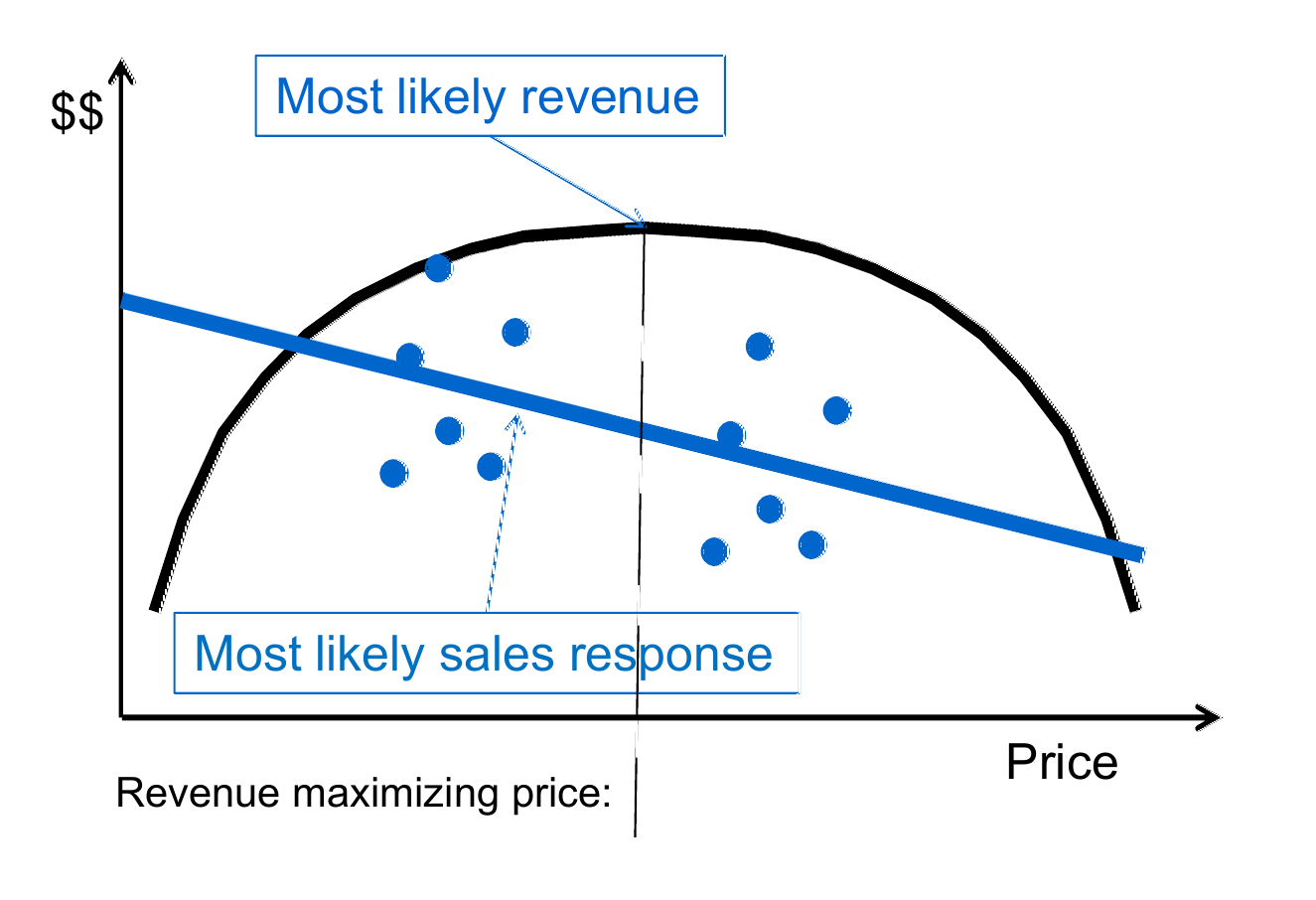
  Figure 7.2 illustrates the challenges of learning a parametric function. Here we show three linear demand response curves giving demand as a function of price with the form $D(p) = \theta_0 - \theta_1 p$. Our goal is to maximize revenue $R(p) = pD(p)$. Figure 7.2(a) shows three possible demand curves and the corresponding revenue curves.

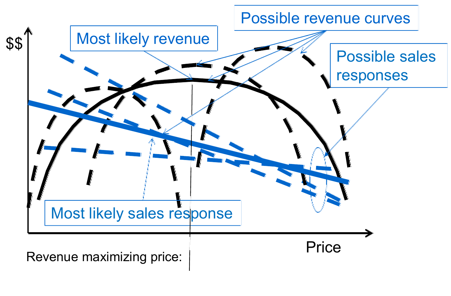
(a)

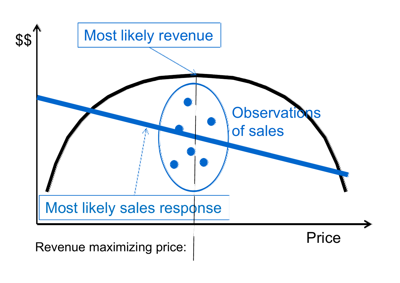
(b)

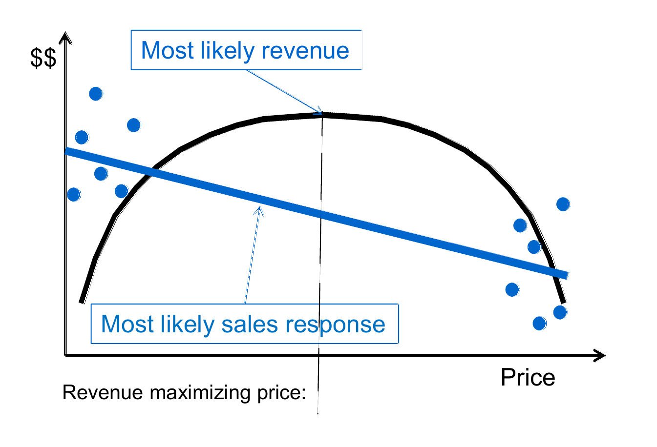
(c)

(d)

It is tempting to want to quote prices that optimize the revenue as we do in Figure 7.2(b), but this produces a set of points in a ball that makes it hard to estimate the demand curve. The best way to estimate the demand curve is to quote prices near the extremes as we do in Figure 7.2(c), but the revenue is very low at these points, so we do not make money while we are learning.

A good approach is to test points on the “shoulders” which means not at the optimum, but not too far away, as we do in Figure 7.2(d), a behavior we accomplish with a policy we describe next.

• Response surface methods with perturbation – A policy that overcomes the exploration vs. exploitation tradeoff illustrated in Figure 7.2 uses a one-step lookahead policy called the knowledge gradient that chooses $x^n$ to be the value that produces the maximum value of information. It turns out the points that maximize the value of information give us the sampling pattern illustrated in Figure 7.2(d).

  The knowledge gradient is too complex for our presentation here, but there is a very simple way of getting the same behavior. Instead of taking our current estimate of the apparent optimum $x^n$ as we do in $\eqref{eq:responsesurfacegreedy}$, we perturb it by an amount $\rho$, but there are two ways of doing this:

  • An optimum-deviation policy – The idea here is to pick a point $x^n$ that is a distance $\rho$ from the optimum $\xbar^n = \argmax_x \Fbar^n(x\vert \thetabar^n)$. If $x$ is a $k$-dimensional vector, this deviation can be created by sampling $k$ normally distributed random variables $Z_1, \ldots, Z_K$, each with mean 0 and variance 1, and then normalizing them so that

    \[\sqrt{\sum_{k=1}^K Z^2_k} = \rho.\]

    Let $\Zbar^n$ be the resulting $k$-dimensional vector. Now compute the sampling point using

    \[x^n_k = \xbar^n_k + \Zbar^n_k.\]

    Note that in one dimension, we would have $\Zbar^n = \pm \rho$.

  • An excitation policy – Here we again generate a $k$-dimensional perturbation vector $Z^n$, where each element has mean 0 and variance 1, and then set

    \[x^n_k = \Xbar^n_k + \rho Z^n_k.\]

    While the optimum-deviation policy forces $x^n$ to be a distance $\rho$ from the optimum $\xbar^n$, an excitation policy simply introduces a random perturbation with mean 0, which means the most likely point to sample is the optimum of $\fbar^n(x\vert \thetabar^n)$.

  We suggest that the optimum-deviation policy is better suited for offline, final-reward objectives, while the excitation policy is better when we are in an online setting optimizing cumulative reward.

What did we learn?

• We review the four classes of policies.
• We use all the applications introduced in the previous six chapters to contrast the different styles of state variables, and to illustrate each of the four classes of policies.
• We also describe final reward and cumulative reward objectives. Final reward objectives arise when we are making observations in an experimental setting (in the lab or the field), where we only care about the performance of the final design. Cumulative reward objectives are used when we are learning while doing.
• We describe both derivative-based and derivative-free search methods for doing parameter search.
• We note that both derivative-based and derivative-free stochastic search are both sequential decision problems.

Exercises

Review questions

1. What distinguishes PFAs from the other three classes of policies?
2. What distinguishes VFAs and DLAs from PFAs and CFAs?
3. In Chapter 1, the state variable for the more complicated inventory problem consists of physical state variables $R_t$, informational state variables $I_t$, and belief state variables $B_t$. What distinguishes a belief state variable from an informational state variable?
4. What is the difference in the objective functions for online and offline learning?
5. We described derivative-based and derivative-free stochastic search as sequential decision problems. Which one of these two strategies uses a belief state, and why is this necessary?

Problem solving questions

1. Figure 7.3 shows a deterministic graph, where we are trying to find a path from node 1 to node 11 using different objectives.
   1. If our traveler simply wants to minimize the total travel time from node 1 to 11, and has currently traversed the path 1-2-6-9, what is her state?
   2. Now assume that our traveler has to arrive at node 11 by time 45. If she arrives after time 45, she is assessed a penalty equal to the square of the delay. What is the state of the traveler who has followed path 1-2-6-9 up to now?
   3. What is the state if the traveler who has followed path 1-2-6-9 wants to minimize the second highest cost on any of the links along her path?

   

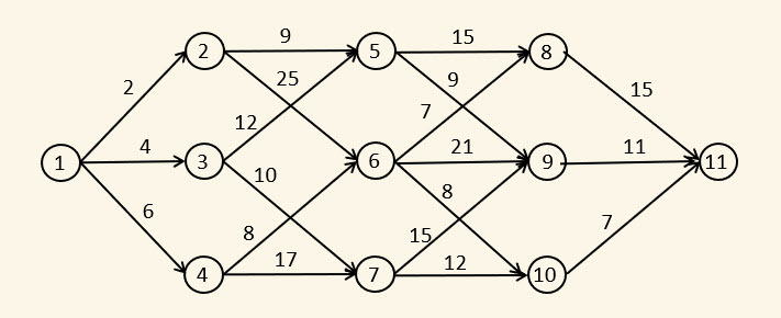
2. Real story: a finance technology company ("fintech") has an algorithmic trading system for high-frequency trading. At time $t$, when an asset is trading at price $p_t$, they estimate whether the price is going up or down using a series of forecasts of how the price might change over a rolling horizon within the day. Here, time is measured in 15-minute increments. Let $f_{tt'}$ be the estimated price of the asset at time $t'$ made given the information at time $t$. Now create an estimated price using $$ \fbar_t(\theta) = \sum_{t'=t+1}^{t+H} \theta_{t'-t} f_{tt'}, $$ where $\theta = (\theta_1, \theta_2, \ldots, \theta_H)$ is the vector of weights for each 15-minute increment for six hours into the future (24 increments). Let $x_t = 1$ indicate a decision to sell at time $t$, $x_t = -1$ is a decision to buy, and $x_t = 0$ is to hold, where the policy is $$ X^\pi(S_t\vert \theta) = \begin{cases} +1 & \text{if } \fbar_t(\theta) \geq p_t + 1.0, \\ 0 & \text{if } p_t - 1.0 < \fbar_t(\theta) < p_t + 1.0, \\ -1 & \text{if } \fbar_t(\theta) \leq p_t - 1.0. \end{cases} $$ The challenge is to optimize the weight vector $\theta$.
   1. At time $t$, what is the state of this system?
   2. What class of policy would $X^\pi(S_t\vert \theta)$ fall in? Explain.
   3. Assume that you can simulate the policy using historical data in a simulator. Let $F(\theta)$ be the expected performance of the policy given parameter vector $\theta$. Write out this objective assuming that you are going to simulate the policy using a single sample of history.
   4. Describe how to compute a numerical derivative using your simulator. Just write the numerical derivative for a single element $\theta_\tau$.