Chapter 11: Supply chain management II: The beer game

Chapter overview

The beer game is a classic in the teaching of supply chain management. We approach it as a general multiagent problem, where each supplier in the beer game is modeled as a separate agent. This presentation extends the foundation we laid in Chapter 10, with the added complication that agents are both sending information (orders for beer) and physical resources (beer).

The chapter keeps the modeling of uncertainty fairly simple. Instead, we explore a series of simple parametric policies, but we use this as an opportunity to introduce beliefs one agent holds about information another agent may have (in this case, about backorders). We then provide an illustration of the well-known “anchor-and-adjustment” policy first introduced by two well-known decision scientists, Daniel Kahneman and Amos Tversky, adapted to the beer game setting. We finish by sketching how we might design a stochastic lookahead policy, exploiting the property that our decision is a scalar.

The chapter closes by proposing an extensive series of extensions, indicating the richness of the variations of control problems that arise in supply chain settings.

Narrative

This chapter covers a famous game from the 1950’s known as the “beer game.” This was originally designed by Jay Forrester, a professor at MIT who created the game to illustrate the instabilities of supply chains. The problem involves a linear supply chain where various suppliers move beer from where it is made (the manufacturer) toward the market (the retailer). The beer has to move through several middlemen on its way from point of manufacture to the market.

There are two types of flows:

• The flow of beer – Each case of beer is represented by a penny that moves from manufacturer to retailer.
• The flow of information – Each point in the supply chain replenishes its inventory by making requests for more beer to the next level down.

Each level of the supply chain is known as an echelon. Typically there are four to six echelons for each team. The demands at the retailer are fixed in advance, but hidden, in a deck of cards. As the retailer reveals that week’s demand, she tries to fill the demand from inventory. The retailer, and every other supplier in the supply chain (other than the manufacturer) then fills out a sheet of paper requesting more inventory.

It is possible that the retailer, or any of the middle suppliers, may not be able to fill the request for more inventory (or the market demand at the retail level). In this case, the unsatisfied demand sits in an order backlog waiting to be filled as new inventory arrives.

After filling orders, everyone (for that supply chain) has to stop and record either their inventory (the number of cases of beer sitting in inventory) or their order backlog. Order backlog carries a penalty of $4 per case. Excess inventory carries a holding cost of $1 per case.

The steps of the process are illustrated in Figure 11.1. There are five steps:

Step 0: Each week, each player will have an inventory (in pennies, each representing a case of beer), and an order, which might be the retail demand (for the retail echelon) or an order placed by the player to their left.

Step 1: Each player tries to take as many cases from their inventory and move it to their left to a point between them and the player to the left (do not add the pennies to the inventory of the player to the left). If there is not enough inventory to satisfy the order, cross out the order and replace it with the number of cases that remain to be satisfied (this is the order backlog).

Step 2: Now write out an order of how many cases you want to replenish your inventory, and place it in the area between you and the player to your right (the manufacturer places an order on the pile of pennies from which all beer originates).

Step 3: Stop and record on your inventory sheet how much inventory you have. If you have not been able to satisfy an order, you will have no inventory, and you will have orders in your backlog (the unsatisfied orders). If this is the case, record this as your order backlog.

Step 4: This is the key step: reach out with your left hand and pull the next order slip into your order pile (the sheets of paper), and at the same time reach out with your right hand to pull the pennies coming to you into your inventory. Now you are back to where you were for step 0.

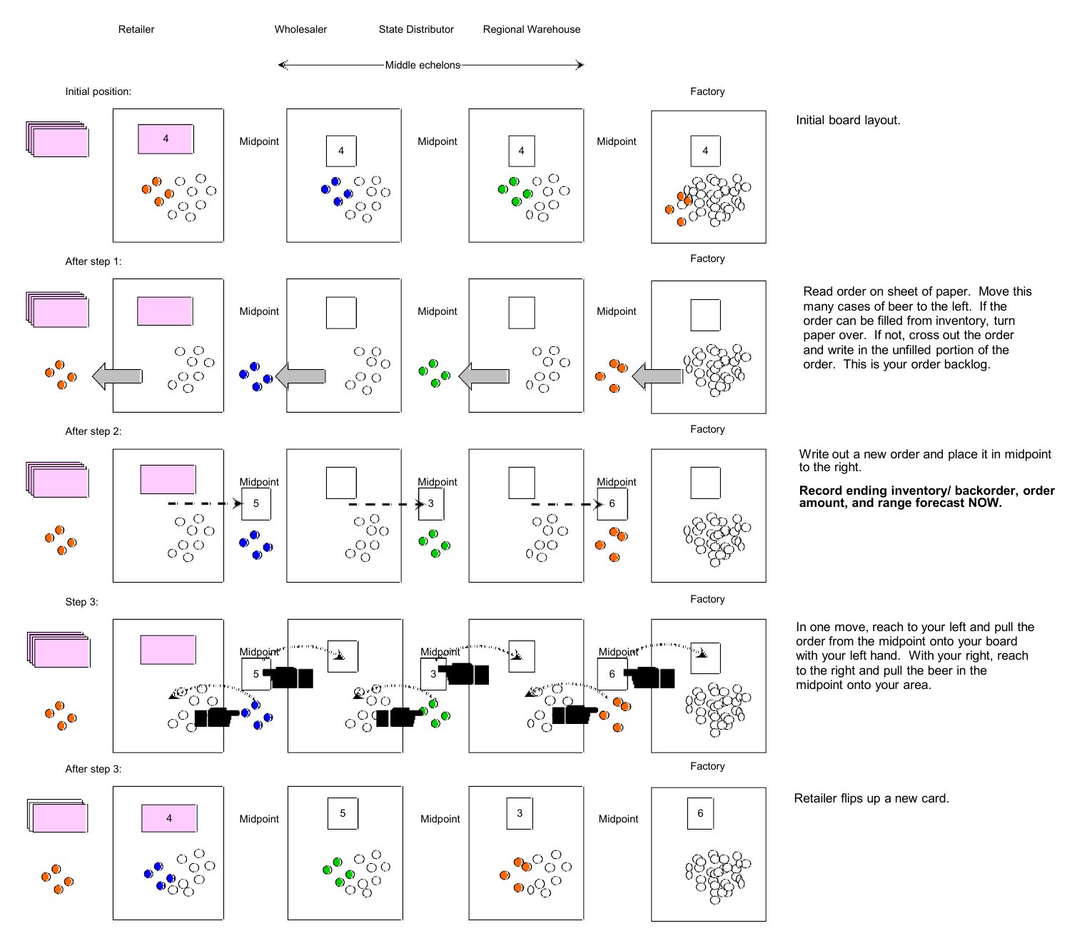
It is very important that everyone make moves at the same time, but they are not allowed to share information (and they should not be looking at the inventories of other players in the same chain). The retailer has to play the role of keeping everyone synchronized.

The complete instructions for a streamlined version of the classic beer game can be downloaded from tinyurl.com/PrincetonBeerGame. This version of the game is ideally suited for classes taught at continuous tables to a class with at least 8-10 students (the continuous tables are needed so players can push paper and pennies between each other). Teams should have five or six players (which means five or six intermediate echelons plus the retailer), but no fewer than four. The person running the inventory closest to the factory may run both positions (since the factory does little more than fill orders). The teams do not have to be the same size, and it is fairly easy to extend a chain to add a late-arriving student. It is possible to run the complete game in a 50 minute lecture.

Framing the problem

This is another multiagent problem. The answers to our three framing questions for each agent are:

• Metrics: Minimize expected inventory holding costs plus backorder costs for unsatisfied orders.
• Decisions: How much new product to request from the next agent along the supply chain.
• Uncertainties: How much the market will request (for the retail agent who directly satisfies the market), or the amount that the next agent closer to the market will order, and the amount of requested orders that are satisfied by upstream agents (closer to the factory).

Basic model

We are going to model a supplier other than one of the endpoints (retailer or beer manufacturer). This model will closely follow the style of the two-agent newsvendor problem in the previous chapter, although there are some adjustments. Before we get started, we have to introduce some new notation for multiagent systems.

Multiagent notation

Before we get started, we need to establish our notational system for who knows what, and the process of sharing information.

We are going to label the different decision-making agents in the supply chain by $\Qcal = {1, 2, \ldots, Q}$. We are going to let $q=0$ describe the market, which is a source of information but does not make decisions. We are going to let $q=Q$ refer to the manufacturing plant which we assume (at least initially) can always make enough product to fill demand.

We start by defining the state variable for agent $q$ using $S_{tq}$, the information known to agent $q$ at time $t$ (this may include beliefs). If agent $q$ acts on agent $q’$, we will use $x_{tqq’}$, the action by agent $q$ on agent $q’$. We note that the decision $x_{tqq’}$ is determined by $q$, but arrives to $q’$ as information.

An action by $q$ on $q’$ at time $t$ may involve the movement of physical resources, but could also include sending information. The action by $q$ on $q’$ will arrive to $q’$ as an exogenous information process arriving to $q’$ at time $t+1$ (which is where any distortions would be captured), which we write as $W_{t+1,q,q’}$, information arriving to agent $q’$ at time $t+1$ from actions taken by agent $q$ (this can be information about resources or one involving the sending or sharing of information from $S_{tq}$).

Finally, there will be times when agent $q$ needs to create an estimate of something known by agent $q’$. If we let $S_{tq’}$ represent something known by agent $q’$, we will let $\overleftarrow{S}{t,q,q’}$ denote the estimate that agent $q$ creates of the information in $S{tq’}$.

State variables

The state variables for agents $q=1, \ldots, Q-1$ are: $R^{inv}{tq}$, the inventory left over after iteration $t$ after delivering product to the upstream vendor for agent $q$; and $R^{back}{tq}$, backordered demand that has not yet been satisfied from inventory.

The manufacturer $q=Q$ is assumed to always have unlimited inventory.

In time we will learn that this is an incomplete statement of the state of the problem, but it is a good starting point.

Decision variables

Agent $q$ has to make two decisions. The first (and most important) is how much to order from the downstream agent $q+1$ which we write as $x^{req}_{tq,q+1}$, the order placed by supplier $q$ to be passed to supplier $q+1$, made at the order instant in iteration $t$, which will be received by $q+1$ to be filled in iteration $t+1$.

The second is how much of the request from the upstream agent to fulfill from inventory. We write this as $x^{fill}{tq,q-1}$, how much of the unsatisfied demand $R^{back}{tq}$ to fill at time $t$ from inventory.

These decisions are constrained for $q=1, \ldots, Q-1$ by:

Constraint $\eqref{eq:beergameconstraint1}$ reflects the reality that we cannot send inventory to agent $q-1$ that we do not have on hand. Constraint $\eqref{eq:beergameconstraint2}$ says we cannot send inventory to agent $q-1$ that has not been requested. Note that $R^{back}_{tq}$ includes new orders that have not yet been filled.

We then write our decision vector as

where our decisions will be made by some policy $X^\pi(S_t)$ which we will design later.

In our basic game, we are always going to fill as much of the order from $q-1$ as we can from inventory, so technically $x^{fill}{tq,q-1}$ is not really a decision since we will just set $x^{fill}{tq,q-1} = \min{R^{back}{tq},R^{inv}{tq}}$. However, it is still an action made by $q$, and it opens the door for richer behaviors later.

If we are the retail market $q=0$, then the request $W_{t,0,1} = x^{req}_{t,0,1}$ made to agent $q=1$ comes from an exogenous information source.

If we are the plant $q=Q$, we always fill the request from $q=Q-1$, so

Exogenous information

There are two types of exogenous information for supplier $q$: $W^{fill}{t+1,q+1,q}$, the amount of product received from supplier $q+1$ in response to the request made at time $t$ but arriving at time $t+1$; and $W^{req}{t+1,q-1,q}$, the order made by supplier $q-1$ at time $t$ of supplier $q$, which would arrive at time $t+1$.

It is important to recognize that the decisions made by agents $q+1$ and $q-1$ come to agent $q$ as exogenous information. This means we could write

We can represent the exogenous information for agent $q$ arriving by time $t+1$ using

This describes the information process for the middle agents $q=1, \ldots, Q-1$. The information process $W_{t,0}$ refers to the market where we assume that there is an exogenous source of requests $x^{req}{t,0,1} = W{t,0,1}$ that are made to agent 1.

Transition function

Our state variables $R^{inv}{tq}$ and $R^{back}{tq}$ for $q=1, \ldots, Q-1$ evolve according to

Equation $\eqref{eq:beergametrans1}$ pulls the request $x^{fill}{t,q,q-1}$ from inventory (it is not allowed to go negative) and then adds incoming inventory $W^{fill}{t+1,q+1,q}$ from the downstream agent $q+1$ to create the inventory at time $t+1$. Equation $\eqref{eq:beergametrans2}$ fills orders that have been requested, held in $R^{back}{tq}$, and then adds new orders $W^{req}{t+1,q-1,q}$ to be filled in period $t+1$.

Objective function

Our objective function for agent $q$ assesses penalties for leftover inventory $R^{inv}{tq}$ and unsatisfied demand $R^{back}{tq}$. Let $c^{inv}_q$ be the unit cost of holding inventory for agent $q$, and $c^{back}_q$ be the unit cost of unsatisfied orders for agent $q$.

These costs are assessed on inventories and backlogged demands after making decisions to fill a customer order but before new orders have arrived. So, our cost function for agent $q$ is given by

Keep in mind that $R^{inv}{tq}$ is the current inventory, so $R^{inv}{tq}-x^{fill}{t,q,q-1}$ is the remaining inventory after we have filled orders for time $t$. Similarly, $R^{back}{tq}$ includes new orders, as well as unfilled orders from previous periods. As a result, $R^{back}{tq}-x^{fill}{t,q,q-1}$ is the orders that were not filled right away.

We now search for the best policy using

This has to be done for each agent $q$, assuming that each are self-optimizing. A separate challenge is choosing policies for each agent, which can only use the information available to each agent, but where we still want policies that achieve a global optimality. That is a question beyond the scope of this book.

Modeling uncertainty

Each agent, other than the agents at the endpoints, has to manage two sources of uncertainty:

• The requests made by the upstream agent, which may be the market, or another agent that is responding in an uncertain way to the demands they face, and the ability of the supply chain to respond to their requests.
• The ability of the upstream agent to fill the orders of the agent.

In other words, the only sources of uncertainty are the market, and the behavior of the agents. The ways in which agents (that are people) interact with each other introduces complex (and uncertain) dynamics. Typically, the game is run where the dynamics of the market is quite modest. Even when it is run this way, human behavior can introduce significant instabilities that have been observed in real supply chains, where they have been given the name “bullwhip effect.”

Designing policies

There are a variety of basic PFA-style policies that we might consider. We start by assuming that we always fill a request up to our available inventory, so

We note that as we design different policies, we may have to introduce additional elements to the state variables to meet the information needs of the policy.

Some simple rules

We are going to warm up with some simple ordering rules:

• Request from agent $q+1$ whatever was requested from $q$ in the previous time period:

This policy ignores how much we have in inventory; it is a pure tracking policy. This policy requires that we store the previous request $W^{req}_{t-1,q-1,q}$ in our state variable which becomes

We then bump it up by $\theta$ to protect against uncertainty.

• Request what is needed to meet current and past requests:

When we have leftover demands, this policy would be double-counting, which means making multiple requests.

• Target inventory policy:

This policy seeks to maintain a specified target inventory $\theta^{target}$ which is not varied as conditions change.

These are basic parameterized PFAs which are easy to implement, but of course require tuning. At the same time, they are quite simple, and ignore factors such as the history of past orders that have not yet been filled (in fact, each of these policies have fundamental flaws).

Keep in mind that $R^{back}{tq}$ is the orders by agent $q-1$ made to agent $q$ which $q$ has not yet filled. The orders placed by $q$ to $q+1$ that have not yet been filled are given by $R^{back}{t,q+1}$, but this is not immediately known to agent $q$. Let $\overleftarrow{R}^{back}{tq,q+1}$ be the estimate of $R^{back}{t,q+1}$ made by agent $q$ of the back-ordered demands known by $q+1$. These are the unfilled orders that $q$ placed to $q+1$, which is a statistic normally maintained by $q+1$.

Normally information known by one agent (such as $q+1$) cannot be known perfectly by another agent (such as $q$), but in this case, this is a statistic that $q$ can maintain on its own using

We can use this statistic to suggest an adjusted target inventory policy, where we are adding the unfilled orders captured by $\overleftarrow{R}^{back}{t+1,q,q+1}$ to our current inventory $R^{inv}{tq}$, which we write using:

• Adjusted target inventory policy:

This policy is a form of PFA (there is no embedded optimization), but it reflects supplies that will be arriving in the future.

An anchor-and-adjustment heuristic

In 1989, John Sterman (MIT professor and expert on business dynamics) wrote a paper applying the principle of “anchor-and-adjustment” developed by Tversky and Kahneman (1974) to the beer game. We are going to outline this idea here.

We begin by defining a set of state variables. The variables we actually use may depend on the policy.

• Physical state variables: $R^{inv}{tq}$, current inventory; $R^{back}{tq}$, backlogged demand; and $R^{transit}{tq}$, current in-transit inventory (we are not capturing how long the inventory has been in transit). The resource state is then $R{tq} = (R^{inv}{tq},R^{back}{tq},R^{transit}_{tq})$.
• Information variables: $F_{t-1,q,q-1}$, actual fill from $q$ to $q-1$ from previous time period, so $F_{t-1,q,q-1} = x^{fill}{t-1,q,q-1}$; and $A{t-1,q+1,q}$, actual arrivals to $q$ from $q+1$ in previous time period, so $A_{t-1,q+1,q} = x^{fill}{t-1,q+1,q}$. The information state is then $I{tq} = (F_{t-1,q-1,q},A_{t-1,q-1,q})$. With these variables we are “remembering” an activity from the previous time period. Their use depends on the policy.
• Belief state variables: $\Abar_{t,q+1,q}$, estimated arrival rate of product from agent $q+1$ (this is an estimate of the rate at which product is arriving to $q$ from $q+1$); $\Fbar_{t,q,q-1}$, estimated fill rate delivered to agent $q-1$ (this is an estimate of the rate at which product is being shipped to $q-1$); and $\Dbar_{t,q-1,q}$, estimated demand rate from $q-1$ (this would equal $\Fbar_{t,q-1,q}$ if we completely filled every order, which means that $\Fbar_{t,q-1,q} \leq \Dbar_{t,q-1,q}$). The belief state is then $B_{tq} = (\Abar_{t,q+1,q},\Fbar_{t,q-1,q},\Dbar_{t,q-1,q})$. As with $I_t$, the use of these variables depends on the policy. Later we are going to propose different ways for computing these estimates.

Our complete state variable is then

The estimated fill rate $\Fbar_{t,q,q-1}$ may be calculated in any of several ways:

• Reactive: $\Fbar_{t,q-1,q} = F_{t-1,q-1,q}$.
• Stable: $\Fbar_{t,q-1,q} = \theta^{trgt-fill}_q$, where $\theta^{trgt-fill}_q$ is a target fill rate set by agent $q$.
• Regressive expectations: $\Fbar_{t,q-1,q} = (1-\gamma)\Fbar_{t-1,q-1,q} + \gamma \theta^{trgt-fill}_q$ for a specified smoothing factor $0 \leq \gamma \leq 1$.
• Adaptive expectations: $\Fbar_{t,q-1,q} = (1-\gamma)\Fbar_{t-1,q-1,q} + \gamma \Fbar_{t,q-1,q}$.

The principle of “anchor-and-adjustment” applied to this setting is to choose an “anchor” which specifies how much we expect we should be ordering on average, with an “adjustment” to reflect current conditions.

• Basic refill policy – We can use any of the methods for computing $\Fbar$ to obtain the policy

• Anchor-and-adjustment policy – We are going to use our estimated order rate $\Fbar_{t,q-1,q}$ as our “anchor,” which is what we expect we should order, but we are going to make adjustments based on our inventory on hand, and inventory in-transit. We represent these adjustments using $\delta R^{inv}{tq}$, the adjustment based on the current inventory $R^{inv}{tq}$; and $\delta R^{transit}{tq}$, the adjustment based on the current in-transit inventory $R^{transit}{tq}$.

  We can use these to create an “anchor-and-adjustment” policy given by

So now we have to design adjustment mechanisms. A possible strategy for $\delta R^{inv}_t$ might be

where $\theta^{inv}_q$ is a smoothing factor and the target inventory $R^{inv-trgt}$ are tunable parameters.

A possible strategy for $\delta R^{transit}_{tq}$ might be

Our vector of tunable parameters would then be

These parameters have to be tuned for each agent $q$.

The anchor and adjustment policy was motivated by human behavior, rather than any justification that it would be near optimal. An advantage is that it is simple, transparent and intuitive. The challenge is always the tunable parameters, and in particular the targets $R^{inv-trgt}$ and $R^{transit-trgt}$, since these are presented as static parameters, when in fact they really need to respond to conditions.

A lookahead policy

We first posed a stochastic lookahead policy in Chapter 7, but we replicate it here for ease of reference:

Equation $\eqref{eq:policiesapproximateDLA2}$ can be particularly daunting. Figure 11.2 illustrates each of the elements in the policy using a basic decision tree (all of this is for a single agent $q$ which we suppress). There is a set of decisions $x_t$ that emanate from the first decision node $S_t$, after which we take an expectation over the random information in $\Wtilde_{t,t+1}$. After that, we use an approximate “lookahead policy” $\Xtilde^{\tilde \pi}(\Stilde_{tt’})$ for each decision node $\Stilde_{tt’}$ in our lookahead model, where we typically simplify the state variable in some way. We also approximate information arriving in the future using $\Wtilde_{tt’}$, either by using a deterministic lookahead model, or a simulated set of possible outcomes.

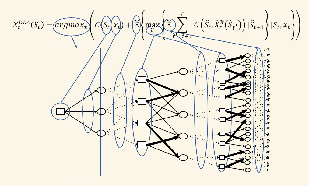
This equation can be thought of as consisting of two elements:

• We first enumerate each possible decision $x_{tq}$.
• Then, we simulate the effects of this decision using a sample of any random information, while making decisions using an approximate “lookahead policy” that is designated $\Xtilde^{\tilde \pi}(\Stilde_{tt’})$.

To use this in our supply chain setting, we have to simulate the behavior of the other agents, realizing that a) we do not know the initial conditions $R_{tq’}$ for $q’ \ne q$, and b) we do not know how the other agents are making decisions.

To handle our lack of knowledge of the starting conditions, we have to view these as random variables and sample from a distribution (this is buried in the first $\Etilde_{\Wtilde_{t,t+1}}$). We note that it is possible for an agent to have, for example, no inventory and a substantial backorder. We might be able to guess that this is the case if we see that the time to fill the orders we are placing are taking a long time to be filled.

We then have to simulate the unknown policies. While we are trying to build a very sophisticated stochastic lookahead policy for agent $q$ at time $t$, we suggest using the much simpler policies we have suggested earlier, not just for the other agents, but also for agent $q$ in future time periods.

So, given these approximations, would a stochastic lookahead policy outperform one of the simpler policies we sketched above? This would be a nice research question, but the lookahead policy overcomes a major limitation of the simpler parametric policies. Specifically, the lookahead policy naturally captures the complex state of this system such as the history of previous orders as well as any forecasts of future events. The parametric policies are suited to stationary problems, while the lookahead naturally adapts to behavior that may be highly nonstationary.

Extensions

There are many ways we can modify this problem. Some ideas include:

1) We have to handle situations where the orders from upstream agents are much bigger (or perhaps smaller) than what we have seen in the past, hinting at a systematic change in demand. We can introduce estimates of the potential growth in future demands to handle unexpected changes in the upstream demand.

2) We can maintain beliefs about how upstream agents might behave. For example, it helps agent $q$ if agent $q+1$ maintains generous inventories. We can encourage inventory building by introducing noise in our own requests which then increase the estimate that agent $q+1$ has of the uncertainty in the orders placed by agent $q$.

3) Each agent reacts to outages, and responds by maintaining higher inventories. An agent $q$ could introduce some noise in their orders to $q+1$ so that $q+1$ will maintain higher inventories so that the orders from $q$ are more likely to be filled.

4) Much of the sensitivity of the game is due to the high penalty for stocking out versus holding inventory (recall that it costs $4 per case per day of backlogged orders, and $1 per case per day to hold inventory). Try changing the stockout cost from $4 to $1, and then to $0.50.

What did we learn?

• We describe a simple multiagent problem called the “beer game” that was invented in the 1950s. To model the problem, we introduce additional notation to capture the knowledge of each agent, and the transfer of information between agents. This can be thought of as a series of two-agent newsvendor problems, with the twist that excess inventory is held to the next time period, as are unsatisfied demands.
• Readers are pointed to a streamlined version of the classic beer game developed by the author at Princeton University.
• We introduce notation that captures what each agent knows, including an estimate by one agent of information known to another agent.
• We model a decision by one agent coming as exogenous information to another agent.
• We begin with some simple PFA policies where agents adapt to basic information on how much they need to order.
• We then summarize a famous “anchor and adjustment” policy suggested by two psychologists, which is another form of PFA.
• Finally we sketch a direct lookahead policy that depends on an agent $q$ simulating the behavior of other agents.

Exercises

Review questions

1. What is the state of an intermediate agent?
2. What decisions can be made by each agent?
3. What are the sources of exogenous information for each intermediate agent?
4. What sources of uncertainty affect the behavior of the game?
5. Explain in words what is meant by an "anchor and adjustment" policy? Was it the expectation of its designers that this might be a good policy?

Problem solving questions

1. Offer a critique of the simple rules suggested above.
2. Imagine that there are occasional, but infrequent, shifts in the demand from the market to much higher or lower levels. Design a policy that understands that these shifts may happen, which means that the rest of the supply chain also has to adapt. How would your policy respond to the invariable periods of shortages of product?
3. The lookahead policy section above provides a rough sketch of a lookahead policy. Fill in the details by writing out an implementation in detail.