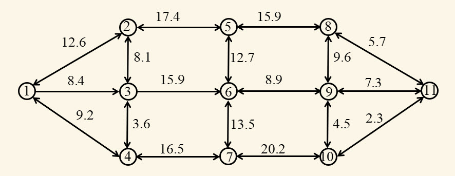
Shortest path problems over graphs are both an important application area (arising in transportation, logistics, and communication), but are also a fundamental problem class that arises in many other settings. The most familiar shortest path problem is the classical deterministic problem illustrated in Figure 5.1, where we have to find the best path from node 1 to node 11, where the cost of traversing each arc is known in advance.
Figure 5.1. Network for a deterministic shortest path problem.
In this chapter we are going to start with a shortest path problem where the travel times are known and fixed. The deterministic version will allow us to demonstrate a particular way of making decisions using Bellman’s equation. We then introduce uncertainty in a very specific way that allows us to demonstrate a solution strategy known as approximate dynamic programming.
Narrative
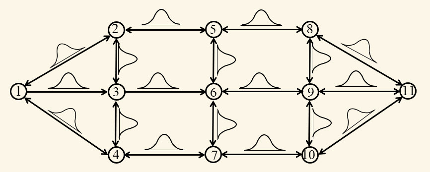
You are trying to create a navigation system that will guide a driverless vehicle to a destination over a congested network. We assume that our system has access to both historical and real-time link costs, from which we can create estimates of the mean and variance of the cost of traversing a link. We can think of this as a shortest path problem where we see distributions rather than actual costs, as depicted in Figure 5.2.
Figure 5.2. Network for a stochastic shortest path problem where distributions are known, but costs are not observed until after decisions are made.
We are going to start by assuming that we have to make decisions of which link to traverse based on these distributions. After we traverse a link from $i$ to $j$, we then experience a sample realization from the distribution. We want to choose a path that minimizes the expected costs.
Framing the problem
The answers to our three framing questions are:
Metrics: We wish to minimize the expected travel time to the destination from the traveler’s origin to a specified destination.
Decisions: When a traveler is at a particular node $i$, they need to make a decision of which downstream node $j$ to traverse to, ultimately leading to the final destination.
Uncertainties: We consider both a deterministic problem, where there is no uncertainty, and a version where the travel times are uncertain but are revealed just before a traveler commits to traversing a particular link.
Basic model
We are going to assume that we are trying to traverse the network in Figure 5.2 starting at a node $q$ and ending at a destination $r$.
Notation
Shortest path problems build on a fundamental dynamic programming recursion. Let $\Ncal$ be the set of all nodes in the network (the nodes $1, 2, \ldots, 11$), $\Ncal^+_i$ be the set of all nodes that can be reached directly from node $i$, $\Ncal^-_j$ be the set of all nodes that are connected to node $j$, $\Lcal$ be the set of all links $(i,j)$ in the network, and $c_{ij}$ be the cost of traversing link $(i,j)$, where $j$ is assumed to be in the set $\Ncal^+_i$.
Let $v_i$ be the minimum cost from node $i$ to the destination node 11. The values $v_i$ for all nodes $i\in\Ncal$ should satisfy
We can execute equation $\eqref{eq:shortestpathbellman1}$ by initializing $v_{11}$ to zero, and setting all other values to some large number. If we loop over every node $i$ and compute $v_i$ using equation $\eqref{eq:shortestpathbellman1}$ repeatedly, the values $v_i$ will converge to the optimal value. This is a very inefficient version of a shortest path algorithm.
Another way to view our network is to assume that each node $i$ is a state $S$, and let $V_t(S_t)$ be the value of being in state $S_t$ at “time” $t$. In our shortest path problem, we are going to use $t$ to index the number of links we have traversed on our way from node 1 to the node represented by $S_t$.
From a state (node) $S_t$, assume we make a decision we call “$x$” which would be a decision to traverse a link emanating from the node corresponding to state $S_t$. We can write this set of decisions as $\Xcal_s$ representing the decisions $x$ that are available to use when we are in state $S_t = s$.
Next let $C(s,x)$ be the cost of being in state $s$ and choosing decision $x$, which would correspond to our link cost $c_{ij}$ in our network above. Finally, we are going to use a “state transition function” that we denote by $S^M(s,x)$ that tells us what state we transition to if we are in state $s$ and take action $x\in\Xcal_s$.
Using this notation, we can rewrite equation $\eqref{eq:shortestpathbellman1}$ as
where $S_{t+1} = S^M(s,x)$. We can execute equation $\eqref{eq:shortestpathbellman2}$ by setting $V_T(s) = 0$ for a large enough value of $T$ (that is, the largest number of links that we might traverse in a path). Since we might set $T$ too large, we have to add to the set of choices in $\Xcal_s$ the ability to stay at the destination node at time $T$. We then set $t=T-1$ and run $\eqref{eq:shortestpathbellman2}$ for all states $s$. We keep repeating this until we get to $t=0$. When we run the system this way, the time index $t$ is really a counter for how many links we have traversed.
Equation $\eqref{eq:shortestpathbellman2}$ is a deterministic version of what is known as Bellman’s equation. In the remainder of this chapter, we are going to show how to use Bellman’s equation to handle uncertainty in our shortest path problem.
State variables
In this basic problem, the state $S_t=N_t$ is the node where we are located after $t$ link traversals. It is tempting to just say the traveler is at node $N_t$, but as we see in the extensions, minor changes produce a richer state variable, and it is important to recognize the true state of our traveler.
Decision variables
We are modeling the decision as the node $j$ that we traverse to given that we are at node $i$. There is a large community that works on problems that fit this class where the decision is represented as an action $a$, where $a$ takes on one of a set of discrete values in the set $\Acal_s$ when we are in state $s$.
A convenient way to represent decisions is to define
\[x_{tij} = \begin{cases} 1 & \text{if we traverse link } i \text{ to } j \text{ when we are at } i, \\ 0 & \text{otherwise.} \end{cases}\]
This notation will prove useful when we write our objective function.
Exogenous information
After traversing the link $(i,j)$, we observe $\chat_{tij}$, the cost we experience traversing from $i$ to $j$ during the $t$th traversal (which we only observe after traversing the link). For the moment, we are going to assume that the new observation $\chat_{tij}$ is stored in a very large database. We can then use these to estimate the average cost $\cbar_{ij}$ of traversing link $(i,j)$ (we exclude the index $t$ for $\cbar_{ij}$ since this is the average cost regardless of when we traverse link $(i,j)$).
Transition function
For our basic graph problem, if we make decision $x_{tij}=1$, the state $N_t = i$ evolves to state $N_{t+1} = j$.
Objective function
We can model our costs using the following notation: $\chat_{tij}$ is a random variable giving the cost to traverse from node $i$ to node $j$; $\cbar_{ij}$ is an estimate of the expected value of $\chat_{tij}$ computed by averaging over our database of past travel costs; and $\sigmabar_{ij}$ is our estimate of the standard deviation of $\cbar_{ij}$ computed using historical data.
We assume that we have to make the decision of which link to traverse out of a node $i$ before seeing the actual value of the random cost $\chat_{tij}$. This means that we have to make our decision using our best estimate of $\chat_{tij}$, which would be $\cbar_{ij}$.
The optimal solution of this problem would be to set all $x_{tij} = 0$, which means we do not get a path. For this reason, we have to introduce constraints of the form
Equations $\eqref{shortestpathobjective1}$–$\eqref{shortestpathobjective5}$ represent a linear program, and there are powerful packages that can be used to solve this problem when written this way. However, there are specialized algorithms (known simply as “shortest path algorithms”) that take advantage of the structure of the problem to produce exceptionally fast solutions.
However, this approach does not provide a method for handling uncertainty. Below, we describe how to solve the stochastic shortest path problem using our language of designing policies, which will provide a foundation for addressing uncertainty.
Modeling uncertainty
For our basic model we are only using the point estimates $\cbar_{ij}$ which we assume is just an average of prior observations collected using, for example, travel cost estimates drawn from GPS-enabled smartphones. When estimates are based on field observations, the method is called data-driven, which means we do not need a model of uncertainty — we just need to observe it.
For example, let $\cbar_{ij}$ be our current estimate of the average travel cost for link $(i,j)$ and assume we just observed a cost of $\chat_{tij}$. We might update our estimate using
where $\alpha$ is a smoothing parameter (sometimes called a learning rate or a stepsize) that is less than 1.
If we update our estimates in this way, then it means that the vector of estimated travel times $\cbar$ is varying dynamically, although we might only do updates once each day, as opposed to within a trip. In our modeling framework, the vector of cost estimates $\cbar$ are captured by the initial state $S_0$. If we let $n$ index the day of the trip, we would let $\cbar^n$ be the cost estimates using the first $n$ days of data, which is then held in the initial state $S^n_0$ when planning for day $n+1$.
Designing policies
Our “policy” for this deterministic problem is a function that maps the “state” (that is, what node we are at) to an action (which link we move over). We can solve this problem by optimizing the linear program represented by equations $\eqref{shortestpathobjective1}$–$\eqref{shortestpathobjective5}$, which gives us the vector $x^\ast _{ij}$ for all links $(i,j)$. We can think of this as a function where given the state (node $i$) we choose an action, which is the link $(i,j)$ for which $x_{ij} = 1$. We can write this policy as a function $X^\pi(S_t)$ using
Alternatively, we can solve Bellman’s equation as we did initially for our deterministic shortest path problem using equation $\eqref{eq:shortestpathbellman1}$. This gives us a value $v_i$ which is the minimum travel cost from each node $i$ to the destination node $r$. Once these values are computed, we can make decisions using the following policy
This means that our “stochastic” shortest path problem can be solved just as we solved our deterministic problem. Below in our extensions, we show that with a minor twist, the situation changes dramatically.
Policy evaluation
Policy evaluation for this problem is not required, because the policy is optimal. Although our link costs are stochastic, as long as we do not learn anything about the actual cost until after we make our decision, the optimal decisions involve solving a deterministic shortest path problem. This will be the last time in this book that we see a problem like this.
Under extensions, we are going to introduce uncertainty in a way that allows us to introduce a powerful algorithmic strategy called approximate dynamic programming (also known as reinforcement learning).
Extension - Adaptive stochastic shortest paths
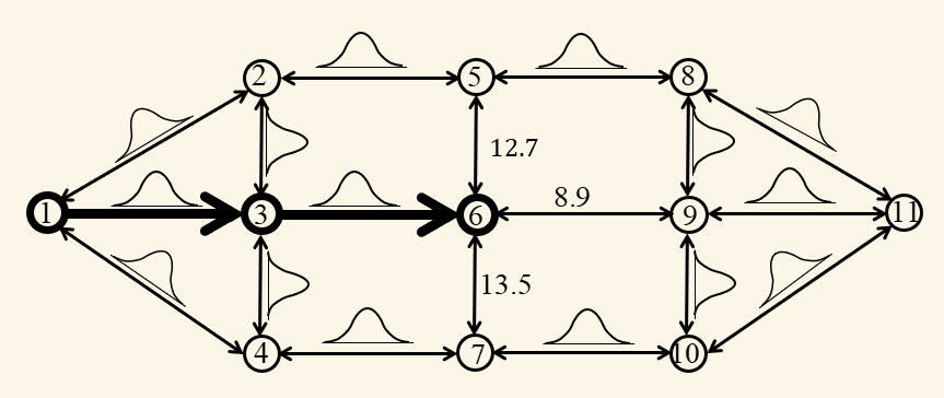
We are going to change the information that we can use while making decisions. In our first stochastic shortest path problem, we assumed that we had to choose the next link to traverse before we see the actual travel cost over the link. Now assume that we make our decision after we observe the link costs, which means we make our decision using the actual cost $\chat_{ij}$ rather than its expectation (or average) $\cbar_{ij}$. This is illustrated in Figure 5.3, where a traveler at node 6 gets to see the actual costs on the links out of node 6 (rather than just knowledge of the distributions).
Figure 5.3. Network for a stochastic shortest path problem where travelers get to see the link costs before making a decision. This graph depicts a traveler who has traversed the path 1-3-6, and now sees the costs on links out of node 6.
If we pretend for the moment that someone can give us the values $v_j$ which is the minimum travel cost from node $j$ to our destination node $r$, an optimal policy for choosing the next downstream node would be written
The problem here is that we cannot compute $v_j$ as we did before using equation $\eqref{eq:shortestpathbellman1}$. In fact, the switch to seeing the costs before we make a decision requires a fundamental change to our basic model.
In our deterministic model, or static stochastic model, the state variable $S_t$ after “$t$” transitions was the node $i$ where the traveler was located. This was the only information we needed at that point in time.
In our new stochastic model, just capturing the node where our traveler is located is no longer enough. Remember that above, we introduced a state variable as “all the information we need at time $t$ from history to model the system from time $t$ onward.” Later, in Chapter 7, we are going to provide a more precise definition, but for now this will serve our needs.
Our new stochastic shortest path problem introduces new information that is needed to make a decision: the costs out of the node where we are located. We are going to find it convenient to introduce two types of state variables: $N_t$, the physical state of the system, which is usually controlled directly by decisions, and $I_t$, other information that we need to make a decision. In our network problem, our physical state would be the node where we are located, while the “other information” variable $I_t$ would capture the costs on links out of the node where we are located, which we write as
\[I_t = (\chat_{tij}), i=N_t, j\in\Ncal^+_i.\]
Assume that at time $t$ that $N_t = i$. We are going to add time $t$ to our index for link costs, which means we will replace $\chat_{ij}$ with $\chat_{tij}$ to refer to the cost when we go from $i$ to $j$ at time $t$. We might then write
To see what this does to our previous way of solving our shortest path problem, take a fresh look at Bellman’s equation as we first introduced it in equation $\eqref{eq:shortestpathbellman2}$ which becomes
where $S_{t+1}$ would be given by $S_{t+1} = (N_{t+1}, I_{t+1})$, where $N_{t+1}$ is the node produced by our decision $x$, so if $x_{ij} =1$, then $N_{t+1} = j$; and $I_{t+1}$ is the costs that are observed out of node $N_{t+1}$, which depends on the decision $x_t$. If $x_t$ sends us to node $j$ so that $N_{t+1} = j$, then $I_{t+1} = (\chat_{t+1,jk_1}, \chat_{t+1,jk_2}, \chat_{t+1,jk_3})$ (assuming there are three links out of node $j$).
Assume that $N_t = i$. The cost function $C(S_t,x)$ is given by
Remember that $S_t$ (where $N_t = i$) contains the costs $\chat_{tij}$ for the links $(i,j)$ out of $i$, so these are known (and contained in $S_t$).
Equation $\eqref{eq:shortestpathbellman5}$ is easy to write but hard to solve now that our state variable is a vector (which explodes the number of states). We are going to first describe two computational challenges. Then, we are going to introduce the idea of the post-decision state to solve one of the two challenges. Finally, we are going to provide a brief introduction to a class of methods known as approximate dynamic programming (but often called reinforcement learning) to handle the second challenge.
Computational challenges
We start by identifying two computational challenges:
The link costs $I_{t+1}$ out of downstream node $N_{t+1}$ (which is determined by the decision $x$) are not known. Said differently, $I_{t+1}$ is a random variable at time $t$, which means we cannot even calculate $V_{t+1}(S_{t+1})$. We fix this by taking the expectation, which we write as
The expectation operator $\E$ should be viewed as taking an average over the possible link costs that a traveler might encounter once they arrive at node $N_{t+1}$ when making decision $x$ (which determines $N_{t+1}$).
To write this more explicitly, assume that $x_t$ sends us to node $j$ (which means that $x_{tij} = 1$), and when we arrive we see $I_{t+1} = (\chat_{t+1,jk_1}, \chat_{t+1,jk_2}, \chat_{t+1,jk_3})$. We learn these costs when we arrive to node $j$ at time $t+1$, but they are random when we are at node $i$ at time $t$ thinking about what to do.
The state space – Even if we assume that the costs $\chat_{t+1,j}$ are discrete, the state space just grew dramatically. Imagine that we have discretized costs into buckets of 20 values. If there are three links out of every node, our state space has grown from the number of nodes, to one that is $20 \times 20 \times 20 = 8,000$ times larger.
To illustrate the challenge of computing the expectation, assume that each cost $\chat_{t+1,jk}$ can take on values $c_1, c_2, \ldots, c_L$ with probabilities $p_{jk}(c_{\ell})$. For example, $c_1$ might be 1 minute, $c_2$ might be 2 minutes, and so on. The probability $p_{jk}(c_{\ell})$ is the probability that $\chat_{t+1,jk} = c_\ell$.
Now assume that the decision $x$ takes us to node $j$, after which we face a choice of traveling over links $(j,k_1), (j,k_2)$ or $(j,k_3)$. We would compute our expectation using
To put it bluntly, equation $\eqref{eq:shortestpathexpectation}$ is pretty ugly. Those triple summations are going to be hard to compute.
Compounding the problem is the size of the state space. To use Bellman’s equation in equation $\eqref{eq:shortestpathbellman6}$ (or $\eqref{eq:shortestpathbellman2}$), we have to compute $V_t(S_t)$ for every possible state $S_t$. When the state was just a node, that is not too bad, even if there are thousands (even tens of thousands) of nodes. However, adding the information variable $I_t$ to the state makes the problem dramatically harder.
To see how quickly this grows the state space, imagine that there are 20 possible values of each cost variable $\chat_{tij}$. That means there are 8,000 possible values of $I_t$. If our network has 10,000 nodes (that is, $N_t$ can take on 10,000 values), then $S_t$ can now take on $10,000 \times 8,000 = 80,000,000$ values.
This is our first peek at what happens when a state variable becomes a vector. The number of possible values of the state variable grows exponentially, a process known widely as the curse of dimensionality.
Using the post-decision state
All is not lost for this problem. There is a trick we can use that allows us to overcome the curse of dimensionality for this particular problem. The main computational challenge with Bellman’s equation in equation $\eqref{eq:shortestpathbellman6}$ is the expectation operator, which is easily the most dangerous piece of notation in solving sequential decision problems.
We are going to use two powerful strategies to overcome this problem in this setting (and we are going to use these strategies for other settings). First, we introduce the idea of the post-decision state which we designate $S^x_t$. The post-decision state is the state of the system immediately after we make a decision, and before any new information arrives, which is why we index it by $t$.
To see pre- and post-decision states, return to Figure 5.3. As we saw before, our pre-decision state (which we call “the state”) $S_t$ is
\[S_t = (6, (12.7, 8.9, 13.5)).\]
Once we have made a decision, we are still at node 6, but imagine that the decision we made was to go to node 9. We might describe our physical post-decision state $R^x_t = 9$, which we might alternatively state as “going to node 9.” However, we no longer need those troublesome observations of costs on the links out of node 6, given by $(\chat_{t+1,6,5}, \chat_{t+1,6,9}, \chat_{t+1,5,7}) = (12.7, 8.9, 13.5)$. This means that our post-decision state is
\[S^x_t = (9).\]
Using the post-decision state, we are going to break Bellman’s equation into two steps. Instead of going from $S_t$ to $S_{t+1}$ to $S_{t+2}$ as we are doing in Bellman’s equation $\eqref{eq:shortestpathbellman6}$, we are going to first step from the pre-decision state $S_t$ to post-decision state $S^x_t$ which we do by rewriting equation $\eqref{eq:shortestpathbellman6}$ as
where $V^x_t$ is the value of being at post-decision state $S^x_t$. Note that we no longer have the expectation, because by construction the post-decision state involves a given decision $x_t$ (e.g. “go to node 9”) but no new information (which is the random part). Note that in this case, the post-decision state $S^x_t$ consists of just the node, which means it is much simpler than $S_t$.
We are not out of the woods. We still have to compute $V^x_t(S^x_t)$, which is done using
So, we still have to compute that expectation, and it has not gotten any easier. Assume that our decision $x$ is to go to node $j$ (which means that $x_{ij}=1$), and let $\chat_{t+1,j} = (\chat_{t+1,jk},~k\in\Ncal^+_j)$ be the set of link costs out of node $j$. Our next pre-decision state $S_{t+1}$ would then be
\[S_{t+1} = (j, \chat_{t+1,j}).\]
Now assume that we have a way of sampling possible values of $\chat_{t+1,j}$. We might do this from a database of historical observations of link costs, or we might build a probability distribution from past data and sample from this. Assume we are going to do this iteratively, and let $\chat^n_{t+1,ij}$ be the $n$th sample of the link cost from $i$ to $j$. We can use this sampling-based strategy to create an estimate of the expectation, rather than the exact value. This is done in the next section.
Approximate dynamic programming
Using post-decision state variables solves the problem of computing the expectation while finding the best decision $x_t$, but we still have the issue of dealing with the large state space. For this, we are going to turn to the methods that are broadly known as approximate dynamic programming, where we replace the post-decision value function $V^x_t(S^x_t)$ with an approximation.
We are going to construct approximations $\Vbar^x_t(j)$ of the value of being at node $j$, where
Let $\Vbar^{x,n}_t(j)$ be our approximation of $\E \lbrace V_{t+1}(S_{t+1})\vert S^x_t\rbrace $ after observing $n$ samples. One way to build this approximation is to use samples of the value of being at node $j$. Imagine that we are going to pass forward through the network, making decisions using approximations $\Vbar^{x,n-1}_t(S^x_t)$ obtained from previous iterations, along with sampled costs $\chat^n_{tij}$. We can obtain a sampled estimate of the value of being in state $S_t$ using
We are then going to use $\vhat^{x,n}_t(i)$, which is the value of being in state $S_t$ (which includes both the node $i$ and the costs $\chat^n_{tij}$ for all $j$ out of node $i$), to update the previous post-decision state $S^x_{t-1}$, which we do using
Here, $\alpha_n$ is known as a smoothing factor or learning rate, but for technical reasons it is also known as a “stepsize.” We might use a constant such as $\alpha_n = .1$ or $.05$, but a common strategy is to use a declining formula such as
\[\alpha_n = \frac{\theta^\alpha}{\theta^\alpha + n - 1},\]
where $\theta^\alpha$ is a tunable parameter. For example, if we set $\theta^\alpha = 1$, we get $\alpha_n = 1/n$. In this case, it is possible to verify that equation $\eqref{eq:vhatsmoothing}$ is averaging over the values $\vhat^n_t(i)$. In practice, this formula is unlikely to work well for this problem because the stepsize goes to zero too quickly.
We pause to note two advantages of the use of the post-decision state $S^x_t$:
We no longer have to deal with the expectation when optimizing over the choice of output links from a node (see equation $\eqref{eq:vhatsinglepass}$).
Approximating the value function $\Vbar^{x,n}_t(S^x_t = i)$ is much simpler since the post-decision state $S^x_t$ is now just a scalar, which is much easier to estimate than a higher-dimensional function.
One challenge with equation $\eqref{eq:vhatsinglepass}$ is that we are going to need initial values for $\Vbar^{x,0}_t(i)$. A natural choice would be to solve the deterministic version of this problem where the costs $\chat_{tij}$ are set equal to estimates of their means, and then obtain initial estimates of the cost incurred to get from each node to the destination.
An alternative method is to use the estimates $\Vbar^{x,n-1}(i)$ to make decisions using
The decision $i^n_t = x^n_t(i)$ gives us the next node after node $i$ based on the sampled costs $\chat^n_{tij}$ and the estimates of the cost $\Vbar^{x,n-1}_t(j)$ to get from node $j$ to the destination node $r$. When we arrive at $r$, we have an entire path consisting of the nodes
\[(q, i^n_1, i^n_2, \ldots, r).\]
We also have the sampled costs $\chat^n_{t,i^n_t,i^n_{t+1}}$ over the entire path. Assume there are $T$ links in the path. We then traverse backward over the path starting with $\vhat^n_T(r) = 0$, and computing
We then use these estimates in our smoothing process in equation $\eqref{eq:vhatsmoothing}$.
This procedure is a form of approximate dynamic programming (alternatively known as reinforcement learning). More specifically, it is a form of forward approximate dynamic programming since it progresses by stepping forward through time. We have illustrated a pure forward pass procedure using equation $\eqref{eq:vhatsinglepass}$, which requires single passes through the network, and a double pass procedure using equation $\eqref{eq:vhatdoublepass}$, which consists of first stepping forward through the graph simulating decisions, and then backward for updating the value of being at each state.
This method is very robust with respect to complex pre-decision states. For example, we do not care how many links might be going out of each node, but we are leveraging the fact that our post-decision state variable is fairly simple (in this case, it is just the node where we are sitting).
What did we learn?
This is the first (and only) time we have a problem where we can find the optimal policy for a sequential decision problem. Although we are optimizing over a stochastic network, the traveler does not receive any advance information about a link before traveling over the link, which means he has to make his choice based on expected costs.
Since the basic model reduces to a deterministic shortest path problem, we can solve this optimally, which is a rare example of being able to solve the base problem optimally (in fact, this is the only time this will happen in this book).
We then introduce the dimension that costs are revealed before the traveler traverses the link. We reformulate the problem, showing that the state variable now becomes much more complex, consisting of the node where the traveler is located and the costs of links out of the node. This problem can no longer be solved exactly using dynamic programming.
We introduce and describe an approximate dynamic programming algorithm using the concept of a post-decision state variable which eliminates the expectation embedded in Bellman’s equation, and reduces the state space back to just the set of nodes.
This is an example of a VFA policy. Since we cannot compute the value functions exactly, we cannot guarantee that it is an optimal policy.
Exercises
Review questions
In the original stochastic shortest path problem where we only observe the actual cost after we traverse the link, explain why this can be solved exactly as a simple deterministic shortest path problem.
For the version where we observe the actual cost over a link before we choose which direction to move, give the pre-decision and post-decision state variables.
In equation $\eqref{eq:vhatsmoothing}$, we use the sampled value $\vhat^{x,n}_t(i)$ of being in state $S_t$ to update the estimated value of being at the previous post-decision state given by $\Vbar^{x,n}_{t-1}(i)$. Create a small numerical example to illustrate this equation.
Problem solving questions
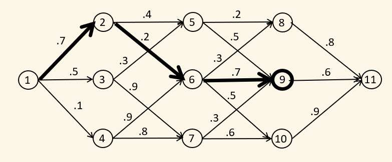
A traveler needs to traverse the graph shown in Figure 5.4 from node 1 to node 11. There is a probability that each link can be traversed, which is shown on the graph (these probabilities are known in advance). When the traveler arrives at node $i$, she gets to see which links (if any) can be traversed out of node $i$. If no links can be traversed, then the trip stops with failure. The goal is to choose a path that maximizes the product of these probabilities, but she is limited to traveling over links that are available.
Describe an appropriate state variable for this problem (with notation).
Imagine the traveler is at node 6 by following the path 1-2-6 and then sees that links 6-9 and 6-10 are available (but 6-8 is not available); what is her (pre-decision) state? I am looking for the numerical values of the state variables you provided in part (a).
Assume that the traveler is able to move to node 9, and decides to do this. What is the post-decision state after making this decision?
Write out Bellman's equation that characterizes the value of being in the pre-decision state after traversing the path 1-2-6 in terms of the downstream pre-decision states. Numerically calculate the value of being in the state after traversing 1-2-6 and observing that 6-9 and 6-10 are available (but 6-8 is not).
Figure 5.4. A shortest path problem to maximize the probability of completing a path.
(This question applies to the adaptive stochastic shortest path extension above.) Write out the steps involved in fitting a value function approximation for the post-decision states by answering:
Write out the pre- and post-decision states. If the network has $N$ nodes, and if the costs on each link are discretized into 20 values (assume at most $L$ links out of any node), what is the size of the pre- and post-decision state spaces?
Give the equation for computing $\vhat^n_t(i)$. Is this the estimate of being at a pre-decision state or a post-decision state? Explain.
What does the "time" index $t$ refer to?
Give the updating equation for updating the value at being at a post-decision state.
Why do we need the value of being at a post-decision state rather than a pre-decision state?
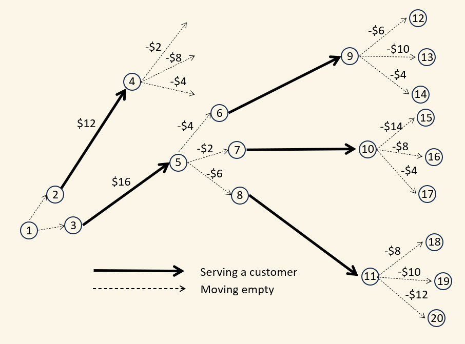
Figure 5.5 illustrates the choices that an Uber driver might face. At node 1, she has a choice of trips (2-4) and (3-5). Assume that trips are at least 15 minutes, and trips are expected to be served within 10 minutes or they are lost. This means the trips out of nodes 6, 7 and 8 only become known after trips (2-4) and (3-5) would have been completed.
Figure 5.5. A decision tree illustrating the choices facing an Uber driver.
Assume that our driver first chooses (3-5) and then chooses (7-10). After completing (7-10), she has to move to a recharging station to charge her battery before returning home (assume she chooses the least cost recharging station).
Alongside each movement is how much she makes (denote this by $c_{ij}$), which is positive for serving a customer and negative for moving empty. Of course she is trying to maximize profits over her entire shift.
The state of our driver is her location (node number) or the node number to which she is headed, along with any other available information known at that time relevant to her decision.
Given that she is initially at node 1, what is her (pre-decision) state? What is her post-decision state after deciding to accept trip (3-5)?
Let $s_1$ be the (pre-decision) state after serving trip (3-5). Let $\vhat_1(s_1)$ be the value of being in state $s_1$. What is $\vhat_1(s_1)$?
Let $s^x_0$ be the previous post-decision state before $s_1$, and let $\vhat^x_0(s^x_0)$ be the value of being in $s^x_0$. What is $\vhat^x_0(s^x_0)$?
What is the computational advantage of using post-decision states over pre-decision states in terms of computing a policy? This should be a one-sentence response.
Programming questions
These exercises use the Python module StochasticShortestPath_Static on tinyurl.com/sdagithub.
(This question applies to the adaptive stochastic shortest path extension above.) Currently the algorithm has a fixed smoothing factor for estimating the value function approximations when solving the modified problem in the extension. Implement a declining stepsize, as follows:
$$
\alpha_n = \frac{\theta^{step}}{\theta^{step} + n-1}.
$$
Run the python module for $\theta^{step} = (1, 5, 10, 20, 50)$ for 100 iterations, and compare the performance in terms of both the rate of convergence and the final solution. Which would you choose?