Chapter 4: Learning the best diabetes medication
Chapter overview
Learning the best diabetes medication picks up where our newsvendor problem left off, where successive time periods are linked by what we believe about unknown parameters. Here, we are trying to learn the best of a set of diabetes medications for a particular patient. We try a medication, observe what we assume is a noisy response, and then update our beliefs to decide what to try next, where we want to maximize the reduction in blood sugar. This problem class has been studied under a variety of names, including multiarmed bandit problem, derivative-free stochastic search, or intelligent trial and error.
At the heart of this problem is our beliefs about how different medications will perform. To keep the presentation as simple as possible, we assume that what we observe from one medication does not tell us anything about the performance of other medications, a property known as independent beliefs. A more interesting and relevant case would capture correlated beliefs, but this would have complicated the presentation.
We consider only the simplest types of policies which are all forms of policy function approximations. These are quite simple to use, but they all involve tunable parameters, which is not addressed in this chapter.
We consider as an extension the case where we want to use what we learn from one patient for other patients with similar attributes. This introduces the attributes of a patient into the state variable, producing what is known as a contextual bandit problem, which means learning the performance of the medication in the “context” of the attributes of the patient. We return to these issues in a much richer problem context in Chapter 12 for the problem of optimizing the choice of URLs to display to maximize ad-clicks.
Framing the problem
The answers to our three framing questions are:
- Metrics: We wish to reduce the patient’s blood sugar (measured by the A1c) down to a target level.
- Decisions: For this chapter, we are just choosing the type of medication to administer (normally we would also need to find the best dosage, but we assume that the dosage is determined by the type of medication and the weight of the patient).
- Uncertainties: How much a medication reduces the patient’s A1c. It may be the case that the patient cannot tolerate a medication, in which case we would set the A1c reduction to zero.
Narrative
When people find they have high blood sugar, typically evaluated using a metric called “A1c,” there are several dozen drugs that fall into four major groups:
- Sensitizers – These target liver, muscle, and fat cells to directly increase insulin sensitivity, but may cause fluid retention and therefore should not be used for patients with a history of kidney failure.
- Secretagogues – These drugs increase insulin sensitivity by targeting the pancreas but often cause hypoglycemia and weight gain.
- Alpha-glucosidase inhibitors – These slow the rate of starch metabolism in the intestine, but can cause digestive problems.
- Peptide analogs – These mimic natural hormones in the body that stimulate insulin production.
The most popular drug is a type of sensitizer called metformin, which is almost always the first medication that is prescribed for a new diabetic, but this does not always work. Prior to working with a particular patient, a physician may have a belief about the potential of metformin, and drugs from each of the four groups, to reduce blood sugar that is illustrated in Figure 4.1.
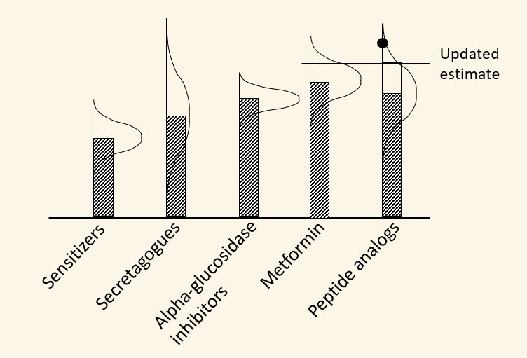
A physician will typically start with metformin, but this only works for about 70 percent of patients. Often, patients simply cannot tolerate a medication (it may cause severe digestive problems). When this is the case, physicians have to begin experimenting with different drugs. This is a slow process, since it takes several weeks before it is possible to assess the effect a drug is having on a patient. After testing a drug on a patient for a period of time, we observe the reduction in the A1c level, and then use this observation to update our estimate of how well the drug works on the patient.
Our challenge is to find a policy for identifying the medication that achieves the greatest possible reduction in a patient’s A1c level.
Basic model
For our basic model, we are going to assume that we have five choices of medications: metformin, or a drug (other than metformin) drawn from one of the four major drug groups. Let $\Xcal = \lbrace x_1, x_2, x_3, x_4, x_5\rbrace $ be the five choices. From observing the performance of each drug over hundreds or thousands of patients, it is possible to construct a probability distribution of the reduction in A1c levels across all patients. The results of this analysis are shown in Table 4.1 which reports the average reduction and the standard deviation across all patients. We assume that the distribution of reductions in A1c across the population is normally distributed, with means and standard deviations as given in the table.
| Drug | A1c reduction | Std. dev. |
|---|---|---|
| Metformin | 0.32 | 0.12 |
| Sensitizers | 0.28 | 0.09 |
| Secretagogues | 0.30 | 0.17 |
| Alpha-glucosidase inhibitors | 0.26 | 0.15 |
| Peptide analogs | 0.21 | 0.11 |
Table 4.1. Metformin and the four drug classes and the average reduction over the full population.
To create a model, let $\mubar^0_x$ be the mean reduction in the A1c for drug choice $x$ across the population, and let $\sigmabar^0_x$ be the standard deviation in the reduction in A1c for drug $x$. Our interest is learning the best drug for a particular individual. Although we can describe the patient using a set of attributes, for now we are only going to assume that the characteristics of the patient do not change our belief about the performance of each drug for an individual patient.
We do not know the reduction we can expect from each drug, so we represent it as a random variable $\mu_x$, where we assume that $\mu_x$ is normally distributed, which we write as
\[\mu_x \sim N(\mubar^0_x, (\sigmabar^0_x)^2).\]We refer to the normal distribution $N(\mubar^0_x, (\sigmabar^0_x)^2)$ as the prior distribution of belief about $\mu_x$.
We index each iteration of prescribing a medication by $n$ which starts at 0, which refers to the time before we have run any experiments. Assume that we always observe a patient for a fixed period of time (say, a month). If we try a drug $x$ on a patient, we make a noisy observation of the true value $\mu_x$ of the patient’s response to a medication. Assume we make a choice of drug $x^n$ using what we know after $n$ trials, after which we observe the outcome of the $n+1$st trial, which we denote $W^{n+1}$ (this is the reduction in the A1c level). This can be written
\[W^{n+1} = \mu_{x^n} + \varepsilon^{n+1}.\]Remember that we do not know $\mu_x$; this is a random variable, where $\mubar^n_x$ is our current estimate of the mean of $\mu_x$.
State variables
Our state variable is our belief about the random variable $\mu_x$ which is the true effect of each drug on a particular patient after $n$ trials. $S^0$ is the initial state, which we write as
\[S^0 = (\mubar^0_x, \sigmabar^0_x)_{x\in\Xcal},\]where we also include in $S^0$ the assumption of normality, which remains through all the experiments. After $n$ experiments, the state is
\[S^n = (\mubar^n_x, \sigmabar^n_x)_{x\in\Xcal},\]where we no longer include the normality assumption because it is captured in our initial state (the distribution is static, so by convention we do not include it in the dynamic state variable).
Later, we are going to find it useful to work with the precision of our belief, which is given by
\[\beta^n_x = \frac{1}{(\sigmabar^n_x)^2}.\]We can then write our state variable as
\[S^n = (\mubar^n_x, \beta^n_x)_{x\in\Xcal}.\]We are using what is known as a Bayesian belief model. In this model, we treat the unknown value of a drug, $\mu_x$, as a random variable with initial prior distribution given by $S^0$. After $n$ experiments with different drugs, we obtain the posterior distribution of belief $S^n$.
Decision variables
The decision is the choice of medication to try for a month, which we write as $x^n$, the choice of medication, where $x^n \in \Xcal = \lbrace x_1, \ldots, x_5\rbrace $. We are going to determine $x^n$ using a policy $X^\pi(S^n)$ that depends only on the state variable $S^n$ (along with the assumption of the normal distribution in $S^0$).
Exogenous information
After making the decision $x^n$, we observe $W^{n+1}_x$, the reduction in the A1c level resulting from the drug $x=x^n$ we prescribed for the $n+1$st trial. A reader might wonder why we write the information learned from the decision $x^n$ as $W^{n+1}_x$ rather than $W^n_x$. We do this to capture the information available in each variable. Thus, the decision $x^0$ depends only on the initial state $S^0$. The state $S^n$ for $n\geq 1$ depends on $S^0$ along with the observations $W^1_{x^0}, \ldots, W^n_{x^{n-1}}$, but not $W^{n+1}_{x^n}$, since we have not yet completed the $n+1$st experiment that would reveal $W^{n+1}_{x^n}$. By letting $W^{n+1}_{x^n}$ be the result of the prescription $x^n$, we know that $x^n$ cannot depend on $W^{n+1}$, which would be like seeing into the future.
Transition function
The transition function captures how the observed reduction in A1c, $W^{n+1}_x$, affects our belief state $S^n$. Although it takes a little algebra, it is possible to show that if we try drug $x=x^n$ and observe $W^{n+1}_x$, we can update our estimate of the mean and precision using
\[\begin{align} \mubar^{n+1}_x &= \frac{\beta^n_x\mubar^n_x + \beta^W W^{n+1}_x}{\beta^n_x + \beta^W},\label{eq:diabetestransition1}\\ \beta^{n+1}_x &= \beta^n_x + \beta^W.\label{eq:diabetestransition2} \end{align}\]where $\beta^W$ is the precision of an observation (we can make this dependent on $x$ if necessary). For all $x\ne x^n$, $\mubar^n_x$ and $\beta^n_x$ remain unchanged.
The transition function, which we earlier wrote as a generic function $S^{n+1} = S^M(S^n,x^n,W^{n+1})$, is given by equations $\eqref{eq:diabetestransition1}$–$\eqref{eq:diabetestransition2}$.
Objective function
Each time we prescribe a drug $x=x^n$, we observe the reduction in the A1c represented by $W^{n+1}_{x^n}$. We want to find a policy that chooses a drug $x^n = X^\pi(S^n)$ that maximizes the expected total reduction in A1c. Our canonical model used $C(S^n,x^n,W^{n+1})$ as our performance metric. For this problem, this would be
\[C(S^n,x^n,W^{n+1}) = W^{n+1}_{x^n}.\]We write the problem of finding the best policy as
\[\begin{align} \max_\pi \E \left\{\sum_{n=0}^{N-1} W^{n+1}_{x^n}\vert S_0\right\}, \label{eq:diabetesobjective1} \end{align}\]where $x^n = X^\pi(S^n)$, and $S^{n+1} = S^M(S^n,x^n,W^{n+1})$. Here, the conditioning on $S_0$ is particularly important because it carries the prior distribution of belief.
Modeling uncertainty
Sampling random outcomes for our asset selling problem was relatively simple. For our medical setting, generating outcomes of the random variables $W^1, \ldots, W^n, \ldots$ is a bit more involved.
With the asset selling problem, we were generating random variables with mean 0 and a given variance which we assumed was known. In this medical application, the reduction in the A1c from a particular drug is a noisy observation of the true mean $\mu_x$ (for a particular patient) which we can write as
\[W^{n+1} = \mu_x + \varepsilon^{n+1},\]where $\varepsilon^{n+1}$ is normally distributed with mean 0 and a variance (which we assume is known) given by $(\sigma^W)^2$. The real issue is that we do not know $\mu_x$. Given what we know after $n$ experiments with different drugs, we assume that $\mu_x$ is normally distributed with mean $\mubar^n_x$ and precision $\beta^n_x$. We write this as
\[\begin{align} \mu_x\vert S^n \sim N(\mubar^n_x, \beta^n_x) \label{eq:mugivenS} \end{align}\]where the right hand side of $\eqref{eq:mugivenS}$ reads “the mean $\mu_x$ given the state $S^n$” which means we assume we know that the mean $\mu_x$ is given by $\mubar^n_x$. We use the precision $\beta^n_x$ (which is one over the variance) instead of the more customary variance when we write our normal distribution. We then write the distribution of $W^{n+1}$ as conditioned on $\mu_x$ using
\[W^{n+1}\vert \mu_x \sim N(\mu_x, \beta^W_x).\]This means that we have to simulate two random variables: the true performance of drug $x$ on our patient, given by $\mu_x$ (given our beliefs after $n$ experiments), and then the noise $\varepsilon^{n+1}$ when we try to observe $\mu_x$. This just means that instead of generating one normally distributed random variable, as we did in our asset selling problem, we have to generate two.
Designing policies
A popular class of policies for this problem class falls in a category known as upper confidence bounding. One of the first UCB policies has the form
\[\begin{align} X^{UCB}(S^n) = \argmax_{x\in\Xcal} \left(\mubar^n_x + 4 \sigma^W \sqrt{\frac{\log n}{N^n_x}}\right), \label{eq:diabetesUCB1} \end{align}\]where $N^n_x$ is the number of times we have tried drug $x$ (recall that “$\argmax_x$” returns the value of $x$ that achieves the maximum). It is standard practice to replace the coefficient $4 \sigma^W$ by a tunable parameter, giving us
\[\begin{align} X^{UCB}(S^n\vert \theta^{UCB}) = \argmax_{x\in\Xcal} \left(\mubar^n_x + \theta^{UCB} \sqrt{\frac{\log n}{N^n_x}}\right). \label{eq:diabetesUCB2} \end{align}\]A popular variant that we have found works surprisingly well was originally introduced under the name interval estimation, which is given by
\[\begin{align} X^{IE}(S^n\vert \theta^{IE}) = \argmax_{x\in\Xcal} \left(\mubar^n_x + \theta^{IE} \sigmabar^n_x \right), \label{eq:diabetesIE} \end{align}\]where $\sigmabar^n_x$ is the standard deviation of the estimate $\mubar^n_x$.
The policies $\eqref{eq:diabetesUCB2}$–$\eqref{eq:diabetesIE}$ both share the structure of choosing the drug $x$ that maximizes our estimate of its performance $\mubar^n_x$ plus a term that is often called an “uncertainty bonus.” The intuition behind these policies is that the estimates $\mubar^n_x$ may be low because of bad luck. Without the uncertainty bonus, a few poor outcomes may mean that we may never try a drug again. These policies have attracted considerable attention from the research literature that can derive theoretical bounds on their performance, but ultimately it all depends on experimental comparisons using realistic data. An important step in the evaluation of the policies is the tuning of the parameter $\theta^{UCB}$ or $\theta^{IE}$.
A third strategy that has attracted considerable attention is known as Thompson sampling. This approach takes a random sample from our belief about $\mu_x$ for each drug $x$, and then takes the best of these. More precisely, let
\[\muhat^n_x \sim N(\mubar^n_x, \theta^{TS} \sigmabar^n_x)\]be a random sample drawn from a normal distribution with mean $\mubar^n_x$ and standard deviation $\sigmabar^n_x$, which is our current belief about the true response $\mu_x$. The parameter $\theta^{TS}$ is a tunable parameter that influences the uncertainty we have around the estimated mean $\mubar^n_x$.
Now choose the drug to try next using
\[\begin{align} X^{TS}(S^n\vert \theta^{TS}) = \argmax_{x\in\Xcal} \muhat^n_x. \label{eq:thompsonsampling} \end{align}\]Thompson sampling favors choices where the estimated performance $\mubar^n_x$, given what we know after $n$ observations (across all drugs), but randomizes the performance. The randomization encourages exploration, since drugs whose estimated impact on A1c may not be the highest, still have a chance of coming out with the highest sampled value $\muhat^n_x$.
We note that all three of these policies, $X^{UCB}(S^n\vert \theta^{UCB})$, $X^{IE}(S^n\vert \theta^{IE})$, and $X^{TS}(S^n\vert \theta^{TS})$, all share two characteristics: the policy itself requires solving an optimization problem (the “$\argmax_x$”), and they all have tunable parameters. For this reason, these are all examples of cost function approximations (or CFAs).
Policy evaluation
We originally wrote our objective function as
\[\max_\pi F^\pi(S_0) = \E \left\{\sum_{n=0}^{N-1} W^{n+1}_{x^n}\vert S_0\right\},\]but writing the expectation in this way is a bit vague. Recall that we have two sets of random variables: the true values of $\mu_x$ for all $x\in\Xcal$, and the observations $W^1, \ldots, W^N$ (or more precisely, the noise when we try to observe $\mu_x$). We can express this nested dependence by writing the objective function as
\[\max_\pi F^\pi(S_0) = \E_\mu \E_{W^1, \ldots, W^N\vert \mu} \left\{\sum_{n=0}^{N-1} W^{n+1}_{x^n}\vert S_0\right\}.\]There are two ways to simulate the value of a policy:
- Nested sampling – First we simulate the value of the truth $\mu_x$ for all $x\in\Xcal$ where we let $\psi\in\Psi$ be a sample realization of $\mu$, which we write as $\mu(\psi)$. We then simulate the observations $W$, where we let $\omega\in\Omega$ be a sample realization of $W^1(\omega), \ldots, W^N(\omega)$, which means that $\omega$ is an outcome of all possible observations over all possible drugs $x\in\Xcal$, over all experiments $n=1, \ldots, N$.
- Simultaneous sampling – Here, we let $\omega$ be a sample realization of both $\mu_x$ and the observations $W^1, \ldots, W^N$.
If we use nested sampling, assume that we generate $K$ samples of the true values $\mu(\psi_k)$, and $L$ samples of the errors $\varepsilon^1(\omega_\ell), \ldots, \varepsilon^N(\omega_\ell)$. For the sampled truth $\mu(\psi_k)$ and noise $\varepsilon^n(\omega_\ell)$, the performance of drug $x^n$ in the $n+1$st experiment would be
\[W^{n+1}_{x^n}(\psi_k,\omega_\ell) = \mu(\psi_k) + \varepsilon^n(\omega_\ell).\]We can then compute a simulated estimate of the expected performance of a policy using
\[\Fbar^\pi(S_0) = \frac{1}{K} \sum_{k=1}^K \left(\frac{1}{L}\sum_{\ell=1}^L \sum_{n=0}^{N-1} W^{n+1}_{x^n}(\psi_k,\omega_\ell)\right),\]where $x^n = X^\pi(S^n)$ and
\[S^{n+1}(\psi_k,\omega_\ell) = S^M(S^n(\psi_k,\omega_\ell), X^\pi(S^n(\psi_k,\omega_\ell)), W^{n+1}(\psi_k,\omega_\ell)).\]If we use simultaneous sampling, then a sample $\omega$ determines both the truth $\mu(\omega)$ and the noise $\varepsilon(\omega)$, allowing us to write a sampled estimate of our observation $W^{n+1}_{x^n}$ as
\[W^{n+1}_{x^n}(\omega_\ell) = \mu(\omega_\ell) + \varepsilon^n(\omega_\ell).\]The estimated value of a policy is given by
\[\Fbar^\pi(S_0) = \frac{1}{L}\sum_{\ell=1}^L \sum_{n=0}^{N-1} W^{n+1}_{x^n}(\omega_\ell).\]If we use one of our parameterized policies where $\theta$ is the tunable parameter, we might write the expected performance as $\Fbar^\pi(\theta\vert S_0)$. Then, the optimization problem would be
\[\begin{align} \max_\theta \Fbar^\pi(\theta\vert S_0), \label{eq:diabetestuningpolicy} \end{align}\]which we can solve using a variety of search procedures such as the methods we presented in this chapter or Chapter 3. We review search methods in more depth in Chapter 7.
Extensions
We have been describing a problem that applies to a single patient. This means that we would have to solve this problem from scratch for each patient. If we have a million diabetes patients, then we would have a million models.
Imagine that we would like to use information from different patients to learn a single model. We can do this by characterizing each patient using a set of attributes $a = (a_1, \ldots, a_K)$. Assume for the moment that each element $a_k$ is discrete (e.g. gender) or discretized (e.g. age, divided into ranges). In fact, we are going to start by assuming that there is a single attribute, gender. Let $G^n$ be the gender of the $n$th patient. Now we have two forms of exogenous information: the gender $G^n$ of the $n$th patient, and the outcome $W^n$ of the treatment of the $n$th patient.
We start with a knowledge state $K^0$ that is our vector $(\mubar^0, \beta^0)$ introduced earlier in the chapter. The first patient will have gender $G^1$, which means our state variable (that is, everything we know) after the first patient arrives is $S^1 = (K^0,G^1)$. We then make a decision $x^1$ regarding the treatment of patient 1, after which we observe an outcome $W^1$ describing how the treatment worked. We use this information to obtain an updated knowledge state $K^1$, after which the process repeats:
\[\begin{align*} &(K^0, G^1, S^1=(K^0,G^1), x^1, W^1, K^{1}, G^2, S^2=(K^1,G^2), \ldots, \\ &\hspace{0.75in} K^{n-1}, G^n, S^n=(K^{n-1},G^n), x^n, W^{n}, K^{n}, G^{n+1}, \ldots) \end{align*}\]We pause for a moment and note that our indexing is different from what we used in the basic model. In our basic model, the index $n$ referred to visits by a patient. We make a decision $x^n$ after the $n$th visit using what is known from the first $n$ visits. We let $W^{n+1}$ be the outcome of this treatment, incrementing $n$ to $n+1$ to emphasize that $x^n$ was computed without knowing $W^{n+1}$.
With our new model, however, $n$ refers to a patient. It makes more sense to let $G^n$ be the gender of the $n$th patient, at which point we make a decision for the $n$th patient, and let $W^n$ be the outcome of the treatment for the $n$th patient. We do not increment $n$ until we see the $n+1$st patient, at which point we see the gender of the $n+1$st patient.
What did we learn?
- We introduced the idea of a sequential decision problem that is a pure learning problem, where the state variable consists only of belief state variables.
- We saw an example of a problem where the uncertainty was in the true value of the performance of a choice such as the diabetes medication.
- We introduced an example of a cost function approximation policy that is a form of parameterized optimization problem, and illustrated this idea using three types of policies: upper confidence bounding (which is a general class of policies), interval estimation, and Thompson sampling.
- We note that each policy involves a tunable parameter and formulate the problem of tuning as its own optimization problem.
- We showed how to model the presence of exogenous information variables (such as the gender of the patient) as a fully sequential decision problem, known in the learning literature as a “contextual bandit problem” (the context is the gender). Instead of finding the best $x$, we are now looking for the best $x(G)$ as a function of gender (we could expand this with other attributes of patients).
Exercises
Review questions
- What is the fundamental difference from an algorithmic perspective between the diabetes problem we solved in this chapter, and the problem solved in [Chapter 3](/sdam/chapter-3/)?
- When we let $\mubar^n_x$ be the estimate of how well the drug performs on a patient after $n$ trials, what is $n$ measuring? Is it the number of times we have tried drug $x$?
- What is the state variable for this problem?
- Above, we introduced an upper confidence bounding policy, an interval estimation policy, and a policy based on Thompson sampling. What characteristics did these policies have in common?
- Did our objective function optimize cumulative reward or final reward? Why did we use that version? What changes if we switch to the other objective function in terms of searching for a good policy?
Problem solving questions
- You are trying to determine the dosage of a diabetes medication that produces the greatest reduction in blood sugar. You are currently experimenting with three dosages that we designate by $d_1$, $d_2$ and $d_3$. Let $\mu_i$ be the true reduction in blood sugar produced by dosage $i$. After $n$ experiments of different drugs, let $\mubar^n_i$ be the estimate of the reduction produced by dosage $d_i$. We wish to exploit the observation that our beliefs about $\mu_i$ are correlated. Let $\sigma_{ii'} = Cov(\mu_i, \mu_{i'})$ be the covariance in our belief about $\mu_i$ and $\mu_{i'}$.
Assume that after $n$ tests of different dosages gives us the current vector of estimates
$$
\mubar^{n} = \begin{bmatrix} 32 \\ 42 \\ 20 \end{bmatrix}.
$$
Assume that the variance of a single experiment is $16$ and that our covariance matrix $\Sigma^n$ is given by
$$
\Sigma^n = \begin{bmatrix} 8 & 4 & 2 \\ 4 & 8 & 4 \\ 2 & 4 & 8 \end{bmatrix}.
$$
- Write out the equations for finding the updated estimates $\mubar^{n+1}$ and covariance matrix $\Sigma^{n+1}$ given an observation $W^{n+1}$.
- Assume that we try dosage $d_2$ and obtain an observation $W^{n+1} = 50$. Compute the updated estimates $\mubar^{n+1}$ and covariance matrix $\Sigma^{n+1}$.
- Show how to adapt the policy presented earlier to our problem where gender is the only patient attribute by using a lookup table representation, which means that instead of learning $\mubar^n_x$, we learn $\mubar^n_{a,x}$ where $a=$ gender. So, instead of learning an estimate $\mubar^n_x$ for each treatment $x$, we have to learn an estimate $\mubar^n_{a,x}$ for each combination of gender $a = G^n$ and treatment $x=x^n$.
- Sketch a strategy for applying the ideas of this chapter to the market planning problem in [Chapter 3](/sdam/chapter-3/).
- Is it possible to apply the methods of [Chapter 3](/sdam/chapter-3/) to the diabetes problem? Explain.
- Now imagine that instead of just gender, we capture age by decade $(0$–$9, 10$–$19, \ldots, 80^+)$, smoker or not, and race (assume eight categories of ethnicity), giving us an attribute vector $a = (a_{gender}, a_{age}, a_{smoker}, a_{race})$. If $a\in\Acal$, how many elements does $\Acal$ have? How would this impact your proposed solution in exercise 7?
- Imagine that each element $a_k$ in the attribute vector $a$ has $L$ possible values, and that $a$ has $K$ elements, which means that $\Acal$ has $L^K$ elements. If $L = 10$, what is the largest value of $K$ so that learning our attribute-based model is easier than learning a model for each of 7 million diabetes patients.
- Now imagine that our attribute space $\Acal$ is simply too large to be practical. What we have done up to now is a lookup table representation where we find an estimate $\mubar^n_{a,x}$, which becomes problematic when the number of possible values of $a$ becomes large. An alternative approach is to use a parametric model. The simplest would be a linear model where we would write
$$
\mubar_{a,x} = \sum_{f\in\Fcal} \theta_f \phi_f(a,x),
$$
where $\phi_f(a,x)$ for $f\in\Fcal$ is a set of features that we (as analysts) would have to define. For example, one feature might just be an indicator of gender, or age range, or race. In this case, there would be a feature for each possible gender, each possible age range, and so on.
- If there are $L$ possible values of each $K$ attributes, what is the minimum number of features we would need?
- Suggest more complex features other than just those that indicate the value of each attribute.
- Contrast the strengths and weaknesses of a lookup table representation versus our linear model.
- We are going to evaluate different policies for finding the best drug for reducing blood sugar. We assume that our prior distribution of belief for each medication is given in Table 4.1.
We begin with a learning policy known as interval estimation given by
$$
X^{IE}(S^n\vert \theta^{IE}) = \argmax_{x\in\Xcal} (\mubar^n_x + \theta^{IE} \sigmabar^n_x).
$$
We use a Bayesian belief model where it is convenient to use the concept of *precision* which is simply one over the variance. So, the precision in our initial estimate of the true value $\mu_x$ is given by
$$
\beta^0_x = \frac{1}{(\sigma^0_x)^2},
$$
where $\sigma^0_x$ is given in Table 4.1.
After $n$ experiments, we are going to use our policy to make a decision $x^n$ which is the drug to try for the $n+1$st experiment. We do not know the true performance $\mu_x$ of drug $x$, but we can observe it using a noisy observation of the true value $\mu_x$ which we write using
$$
W^{n+1}_x = \mu_x + \varepsilon^{n+1}_x.
$$
Assume that the standard deviation of a single experiment is $\sigma^W = 5$. We use the observation of $W^{n+1}_x$ to update our beliefs using:
- If we try drug $x$: $$ \mubar^{n+1}_x = \frac{\beta^n_x \mubar^n_x + \beta^W W^{n+1}_x}{\beta^n_x + \beta^W}, \qquad \beta^{n+1}_x = \beta^n_x + \beta^W. $$
- If $x$ is a drug we do not try, then: $$ \mubar^{n+1}_x = \mubar^n_x, \qquad \beta^{n+1}_x = \beta^n_x. $$
- Using a Bayesian belief model, what is the state variable?
- What is the transition function for the belief model?
- Write out the expected value of a policy $X^\pi(S^n)$ using the expectation operator $\E$. Be sure to index the operator to indicate which random variables are involved, as in $\E_\mu$ or $\E_W$ (or $\E_{W_1,\ldots,M}$). You can show conditioning by using $\E_{W\vert \mu}$ (this is the expectation over the observed reduction $W$ given we know the true mean $\mu$).
- We might reasonably think that the parameter $\theta^{IE}$ should depend on the number of experiments remaining in our budget, which means that $\theta^{IE}$ needs to be a function of $n$ (or equivalently, it would be a function of the remaining experiments $N-n$). There are two ways to represent this function. Discuss (without any programming) the strengths of each approach, and the computational challenges that would be involved.
- Lookup table – Instead of searching over a scalar $\theta^{IE}$, we would have to search over a vector $\theta^{IE}_n$.
- Parametric – We might assume a function form such as $\theta^{IE} = \theta^{slope}(N-n)$, where now we just have to tune the scalar $\theta^{slope}$.
- We have approached this problem as if we are solving the problem for each patient. Imagine that we have $I$ patients indexed by $i = 1, \ldots, I$, remembering that $I$ might be 10 million patients. Finding a vector of estimates $\mubar = (\mubar_x)_{x\in\Xcal}$ for each patient would be written $\mubar = (\mubar_{i})_{i=1}^I$ where each $\mubar_i = (\mubar_{ix})_{x\in\Xcal}$. Creating 10 million estimates seems a bit clumsy.
Imagine instead that each patient has a vector of attributes $a = (a_1,\ldots, a_M)$ where $a \in \Acal$. There may be a lot of attributes, in which case the set $\Acal$ would be quite large, but we may choose a small subset so that $\Acal$ is not as big, such as gender and whether they smoke. We can again use two different representations of $\mubar_{ax}$. As before, discuss the strengths and computational challenges of each of the following ways of modeling $\mubar_{ax}$:
- Lookup table – We would enumerate each of the attributes $a \in \Acal$, and create an estimate $\mubar_{ax}$ of the performance of each drug $x$ and for each attribute $a$. This might be a large set, but should be smaller than 10 million.
- Parametric – This requires coming up with a parametric form for $\mubar_{ax}$ for each drug $x$. One might be $$ \mubar_{ax} = \sum_{f\in\Fcal} \thetabar_{fx} \phi_f(a). $$ The functions $\phi_f(a)$ are sometimes called basis functions (other terms are independent variables or covariates). These might be indicator variables that capture, for example, the gender of the patient or whether they are a smoker. This representation replaces computing $\mubar_{ax}$ for each attribute $a$ with computing a vector of coefficients $\mubar_{ax}$ for a set of features. The set $\Fcal$ is presumably much smaller than the set of attributes (if this is not the case, then we should use the lookup table representation).
Programming questions
These exercises use the Python module AdaptiveMarketPlanning on tinyurl.com/sdagithub.
- Perform $L = 1000$ simulations of the interval estimation policy over a budget of $N = 20$ experiments using $\theta^{IE} = 1$. Let $\Fhat^{IE}$ be the performance of the IE policy for a particular sample path. Make the assumption that the true performance of a drug, $\mu_x$, is given in Table 4.2, and use the assumptions for the standard deviation of each belief from Table 4.1. Also use the standard deviation $\sigma^W = 5$ for the experimental variation as we did in exercise 13.
- Compute the mean and standard deviation of the value of the policy $\Fbar^{IE}(\theta^{IE})$ with $\theta^{IE}=1$.
- Evaluate the IE policy for $\theta^{IE} = (0, 0.2, 0.4, \ldots, 2.0)$ and plot $\Fbar^{IE}(\theta)$. What do you learn from this plot?
- Evaluate the IE policy given a budget $N = 20$ over the values $\theta^{IE} = (0, 0.2, 0.4, \ldots, 2.0)$ for two different sets of truths:
- First assume that the prior is $\mu^0_x = 0.3$ for all drugs $x$ and where the initial standard deviation $\sigma^0_x = 0.10$. This means we are assuming that the truth $\mu_x \sim N(\mubar^0_x,(\sigmabar^0_x)^2)$. However, we are going to sample our truth using $$ \muhat_x = .3 + \varepsilon $$ where $\varepsilon$ is uniformly distributed in the interval $[-0.15,+0.15]$. This is an example of having a prior distribution of belief (in this case, that is normally distributed around 0.3) but sampling the truth from a different distribution (that is uniformly distributed around the mean 0.3). Perform 10,000 repetitions of each value of $\theta^{IE}$ to compute the average performance. What conclusions can you draw from the resulting plot over the 11 values of $\theta^{IE}$?
- For this exercise we are going to simulate our truth from the prior using $$ \mu_x = \mubar^0_x + \varepsilon $$ where $\mubar^0$ is given in Table 4.2 ("A1c reduction") and where $\varepsilon$ is uniformly distributed in the interval $[-.5\mubar^0_x, +.5\mubar^0_x]$. Perform 10,000 repetitions of each value of $\theta^{IE}$ to compute the average performance. What conclusions can you draw from the plot?
| Drug | A1c reduction | Truth |
|---|---|---|
| Metformin | 0.32 | 0.25 |
| Sensitizers | 0.28 | 0.30 |
| Secretagogues | 0.30 | 0.28 |
| Alpha-glucosidase inhibitors | 0.26 | 0.34 |
| Peptide analogs | 0.21 | 0.24 |
Table 4.2. True values for a particular patient.