Chapter 3: Adaptive market planning

Chapter overview

We use the term “adaptive market planning” to describe what is widely known as the newsvendor problem, where we have to choose a quantity of a resource to sell (the “newspapers”) to meet an unknown market demand, where unused resources are discarded at the end of the selling period. This means that different time periods are not physically connected.

We start by using this problem to illustrate a basic stochastic gradient algorithm which is known to converge to the optimal quantity. This approach overcomes the problem that if we allocate too little, we do not observe the actual demand, but instead just how much we are able to sell (which is limited by the inventory we made available).

Stochastic gradient algorithms are widely used when optimizing under uncertainty, where we have access to a gradient. Stochastic gradient algorithms were first introduced in 1951 and enjoy well-understood convergence properties. Less well known, however, is the idea that a stochastic gradient algorithm is itself a sequential decision problem, where the “decision” is the stepsize used in the algorithm.

The classical literature on stochastic gradient algorithms focuses on the property that in the limit, they will produce the optimal solution to a single-period problem (that is, they find the optimal quantity to allocate). Almost entirely overlooked is that when this is done in a field setting, which means we are experiencing the results as they happen, we have to use as our objective the task of maximizing the cumulative reward which is the sum of rewards over time.

In the extensions, we also introduce a twist that is overlooked in the literature. In practice, we not only do not know the demand, we do not even know the distribution of demand. Each time period, we observe how much we sell (which is limited by the quantity of the resource we make available), and we learn from this experience to update our belief about the distribution before we decide how much to allocate in the next time period. This introduces a belief state that links the time periods together, just as would happen if we keep the left over inventory to the next time period. This is another perspective that is missing from classical treatments of the newsvendor problem.

These issues offer considerable richness to what is still a fairly simple and elegant sequential decision problem.

Framing the problem

The answers to our three framing questions are:

• Metrics: Maximizing the expected revenue from meeting demand, minus the cost of purchasing the product, over a planning horizon.
• Decisions: How much product to purchase each time period.
• Uncertainties: The demand for the product in each time period.

Narrative

There is a broad class of problems that involve allocating some resource to meet an uncertain (and sometimes unobservable) demand. Examples include:

• Stocking a perishable inventory (e.g. fresh fish) to meet a demand where leftover inventory cannot be held for the future.
• Stocking parts for high-technology manufacturing (e.g. jet engines) where we need to order parts to meet known demand, but where the parts may not meet required specifications and have to be discarded. So, we may need to order eight parts to meet the demand of five because several of the parts may not meet required engineering specifications.
• We have to allocate time to complete a task (such as driving to work, or allocating time to complete a project).
• We have to allocate annual budgets for activities such as marketing. Left-over funds are returned to the company.

The simplest problem involves making these decisions to meet an uncertain demand with a known distribution, but the most common applications involve distributions that are unknown and need to be learned. There may be other information such as the availability of forecasts of the demand, as well as dynamic information such as the market price for the fresh fish (which may be known or unknown before the resource decision is made).

This problem has been widely studied since the 1950’s, originally known as the “single period inventory problem” but currently is primarily identified as the “newsvendor problem.” It is widely used as the canonical problem in optimization under uncertainty.

The newsvendor problem is typically formulated as

where $x$ is our decision variable that determines the amount of resource to meet the demand, and where $W$ is the uncertain demand for the resource. We assume that we “purchase” our resource at a unit cost of $c$, and we sell the smaller of $x$ and $W$ at a price $p$ (which we assume is greater than $c$). The objective function given in equation $\eqref{eq:newsvendorasymptotic}$ is called the asymptotic form of the newsvendor problem.

There are two important variations of the newsvendor problem:

• The distribution of the random variable $W$ is known.
• The distribution of $W$ is unknown.

The unknown case is what arises more often in practice, which introduces the dimension that each time we run an iteration of choosing $x$ and then observing the smaller of $x$ and $W$, we learn something about the distribution of $W$.

If $W$ was deterministic (and if $p > c$), then the solution is easily verified to be $x = W$. Now imagine that $W$ is a random variable with probability distribution $f^W(w)$ ($W$ may be discrete or continuous). Let $F^W(w) = Prob[W \leq w]$ be the cumulative distribution of $W$. If $W$ is continuous, and if we could compute $F(x) = \E F(x,W)$, then the optimal solution $x^\ast $ would satisfy

Now consider what is known as the stochastic gradient, where we take the derivative of $F(x,W)$ assuming we know $W$, which is given by

This is a gradient (that is, a derivative) of $F(x,W)$ given the random variable $W$, which is “stochastic” because it depends on the random variable $W$ which is revealed only after we choose $x$. This is the reason that $d F(x,W)/dx$ in equation $\eqref{eq:newsvendorstochasticgradient}$ is called a “stochastic gradient.”

Taking expectations of both sides of $\eqref{eq:newsvendorstochasticgradient}$ gives

We can now solve for $F^W(x^\ast )$ giving

Thus, as $c$ decreases to 0, we want to order an amount $x^\ast $ that will satisfy demand with probability 1. As $c$ approaches $p$, then the optimal order quantity will satisfy demand with a probability approaching 0.

This means that we compute $(p-c)/p$, which is a number between 0 and 1, and then find the quantity $x^\ast $ that corresponds to the order quantity where the probability that the random demand is less than $x^\ast $ is equal to $(p-c)/p$.

We have just seen two situations where we can find the order quantity exactly: when we know $W$ in advance (we might call this the perfect forecast) or when we know the distribution of $W$. This result has been known since the 1950’s, sparking a number of papers for estimating the distribution of $W$ from observed data, handling the situation where we cannot observe $W$ directly when $x < W$ (that is, we only observe sales, rather than demand, a situation known as “censored demands”).

We are going to tackle the problem where the demand distribution is unknown. Our approach will be to use a sequential search algorithm given by

where $\alpha_n$ is known as a stepsize. Our challenge will be to choose $\alpha_n$ at each iteration.

Basic model

State variables

The state variable captures the information we have at time $n$ that we need, along with the policy and the exogenous information, to compute the state at time $n+1$. For our search procedure in equation $\eqref{eq:stochasticgradientalgorithm}$, our state variable is given by

Decision variables

The trick with this problem is recognizing the decision variable. It is tempting to think that $x^n$ is the decision, but in the context of this algorithm, the real decision is the stepsize $\alpha_n$. As with all of our sequential decision problems, the decision (that is, the stepsize) is determined by what is typically referred to as a stepsize rule, but is sometimes called a stepsize policy that we denote by $\alpha^\pi(S^n)$.

Normally we introduce policies later, but to help with understanding the model, we are going to start with a basic stepsize policy called a harmonic stepsize rule given by

This is a simple deterministic stepsize rule, which means that we know in advance the stepsize $\alpha_n$ once we know $n$. Below we introduce a more interesting stochastic stepsize policy that requires a richer state variable.

We are also going to let $X^\pi(S^n)$ be the value of $x^n$ determined by stepsize policy $\alpha^\pi(S^n)$.

Exogenous information

The exogenous information is the random demand $W^{n+1}$ for the resource (product, time or money) that we are trying to meet with our supply of product $x^n$. We may assume that we observe $W^{n+1}$ directly, or we may just observe whether $x^n \leq W^{n+1}$, or $x^n > W^{n+1}$.

Transition function

The transition equation, for the setting where $x$ is unconstrained, is given by

We note that it is possible that equation $\eqref{eq:stochasticgradientaltransition1}$ produces a value $x^{n+1} < 0$, which cannot be implemented. The fix here is simple: just set $x^{n+1} = 0$.

Objective function

At each iteration we receive a net benefit given by

Now we have to construct an objective function to find the best policy. We can approach this problem setting in two ways. In the first, we assume that we have to learn in the field, while the second assumes that we have access to a simulator for learning the policy.

Optimizing in the field

If we are experiencing our decisions in the field, we want to maximize the cumulative reward over some horizon. This means we need to find the best policy (which in this setting means the best stepsize rule) by solving

where $S^{n+1} = S^M(S^n,X^\pi(S^n),W^{n+1})$ describes the evolution of the algorithm (for example, the transition function given by equation $\eqref{eq:stochasticgradientaltransition1}$). Here, $\pi$ refers to the type of stepsize rule (we consider several below), and any tunable parameters (such as $\theta^{step}$).

Oddly, the story behind the newsvendor problem always involves learning in the field, and yet the cumulative reward in equation $\eqref{eq:newsvendorobjectivecumulativereward}$ is never used as the objective function. We mention this for readers who do a literature search on the “newsvendor problem.”

Optimizing using a simulator

Alternatively, we might be using a simulator where we are going to run our search for $N$ iterations, ending with $x^N$. We are going to rename this final solution $x^{\pi,N}$ to express the dependence on the stepsize policy $\alpha^\pi(S^n)$.

Our final solution $x^{\pi,N}$ is a random variable since it depends on the sequence $W^1, \ldots, W^n$. As before, we are going to let $\omega$ represent a sample realization of $W^1(\omega), \ldots, W^n(\omega)$, and we write our solution as $x^{\pi,N}(\omega)$ to indicate that this is the solution we obtained when we used the sample path $\omega$.

Since we are using a simulator, we only care about the performance of the final solution (also called the final reward), which we write as

where $\What$ is a random variable that we use for testing the performance of $x^{\pi,N}$.

This means we have two random variables in our objective function given in $\eqref{eq:newsvendorxpiNobjective}$. For a single set of realizations of $W^1(\omega), \ldots, W^n(\omega)$, we get a solution $x^{\pi,N}(\omega)$. Now let $\psi$ be a sample realization of $\What$. So, if we have a sample realization of the solution $x^{\pi,N}(\omega)$, and a sample realization of our testing variable $\What(\psi)$, our performance would be

What we really want to do is to take averages over the possible realizations of both $x^{\pi,N}(\omega)$ and $\What(\psi)$, which we can write using

The estimate $\Fbar^\pi$ represents an average over $N$ samples of the sequence $W^1(\omega), \ldots, W^n(\omega)$, and $M$ samples of the testing variable $\What(\psi)$.

Uncertainty modeling

Let $f^W(w)$ be the distribution of $W$ (this might be discrete or continuous), with cumulative distribution function $F^W(w) = Prob[W \leq w]$. We might assume that the distribution is known with an unknown parameter. For example, imagine that $W$ follows a Poisson distribution with mean $\mu$ given by

We may assume that we know $\mu$, in which case we could solve this problem using the analytical solution given at the beginning of the chapter. Assume, instead, that $\mu$ is unknown, but with a known distribution $p^\mu_k = Prob[\mu=\mu_k]$. Note that this distribution $p^\mu = (p^\mu_k)_{k=1}^K$ would be modeled in our initial state $S^0$.

Designing policies

We have already introduced two choices of stepsize policies which we write as $\alpha^\pi(S^n)$ to mimic our style elsewhere for writing policies.

A wide range of stepsize policies (often called stepsize rules) have been suggested in the literature. One of the simplest and most popular is the harmonic stepsize policy given by

Figure 3.1 illustrates the behavior of the harmonic stepsize rule for different values of $\theta^{step}$.

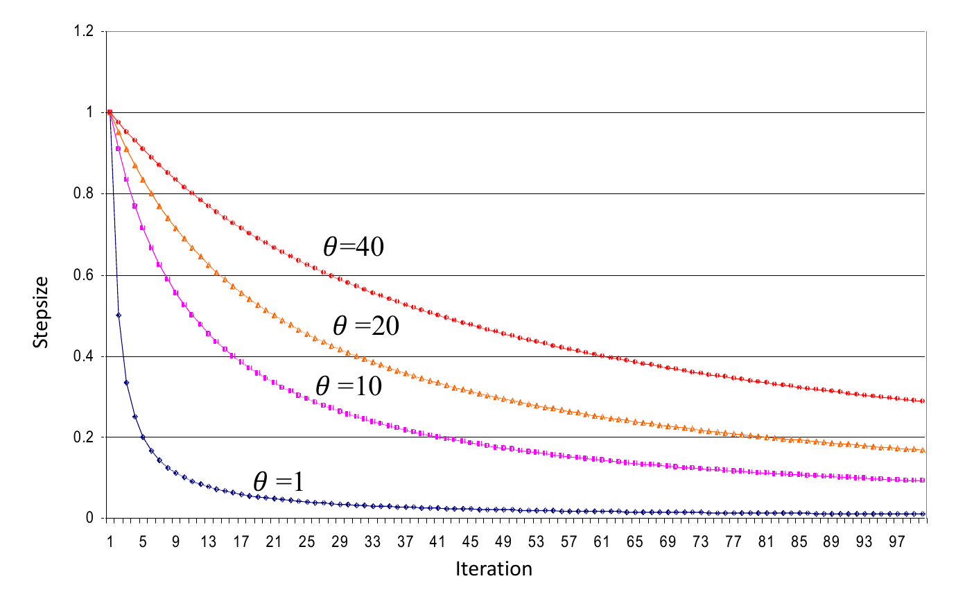
The harmonic stepsize policy is also known as a deterministic policy, because we know its value for a given $n$ in advance. The challenge with deterministic policies is that they are not allowed to adapt to the data. For this reason, it is often useful to use a stochastic rule. One of the earliest and simplest examples is Kesten’s rule

where $K^n$ is a counter that counts how many times the gradient has switched direction. We determine this by asking if the product (or inner product, if $x$ is a vector) $(\nabla_x F(x^n,W^{n+1}))^T \nabla_x F(x^{n-1},W^n) < 0$. If the gradient is switching directions, then it means that we are in the vicinity of the optimum and are stepping past it, so we need to reduce the stepsize. This formula is written

where $\nabla_x F(x^n,W^{n+1}) = \frac{d F(x,W^{n+1})}{dx}$.

Now we have a stepsize that depends on a random variable $K^n$, which is why we call it a stochastic stepsize rule. If we use Kesten’s rule, we have to modify our state variable to include $K^n$, giving us

We also have to add equation $\eqref{eq:kestenupdate}$ to our transition function.

Another stepsize rule, known as AdaGrad, is particularly well suited when $x$ is a vector with element $x_i,~i=1, \ldots, I$. To simplify the notation a bit, let the stochastic gradient with respect to element $x_i$ be given by

Now create an $I \times I$ diagonal matrix $G^n$ where the $(i,i)$th element $G^n_{ii}$ is given by

We then set a stepsize for the $i$th dimension using

where $\theta$ is a tunable parameter (comparable to $\theta^{step}$ in our harmonic stepsize formula) and $\epsilon$ is a small number (e.g. $10^{-8}$ to avoid the possibility of dividing by zero).

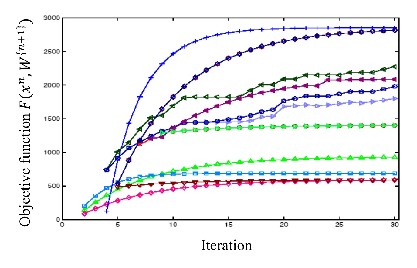
Figure 3.2 illustrates different rates of convergence for different stepsize rules, showing $F(x^n,W^{n+1})$ as a function of the number of iterations. If we were optimizing the final reward in $\eqref{eq:newsvendorxpiNobjectivesampleaverage}$, we could just pick the line that is highest, which depends on the budget $N$. If we are optimizing the cumulative reward in equation $\eqref{eq:newsvendorobjectivecumulativereward}$, then we have to focus on the area under the curve, which favors rapid initial convergence.

Extensions

1) Imagine that we do not know $\mu$, but let’s assume that $\mu$ can take on one of the values $(\mu_1, \mu_2, \ldots, \mu_K)$. Let $H^n$ be the history of observations up through the $n$th experiment, and let $H^0$ be the initial empty history. We assume we start with an initial prior probability on $\mu$ that we write as

After we have observed $W^1, \ldots, W^n$, we would write our updated distribution as

We can update $p^n = (p^n_k)_{k=1}^K$ using Bayes theorem

where

With this extension to the basic model, we have two probability distributions: the belief on the true mean $\mu$, and the random demand $W$ given $\mu$. To include this extension, we would have to insert $p^n$ into our state variable, so we would write

2) Imagine that our problem is to purchase a commodity (such as oil or natural gas) in month $n$ to be used during month $n+1$. We purchase the commodity at a unit cost $c$, and sell it up to an unknown demand $D^{n+1}$ at an unknown price $p^{n+1}$. We would write our objective for this problem as

What did we learn?

• We used the context of a newsvendor problem to illustrate a stochastic gradient algorithm as a sequential decision problem. We showed how to model a stochastic gradient algorithm using the five elements of a sequential decision problem introduced in Chapter 1.
• We introduced several examples of PFA policies for choosing the stepsizes.
• The newsvendor problem is classically stated as a static problem where we search for the best solution where we are only interested in the performance of our final choice of $x$. In this chapter, we introduced two objectives: the cumulative reward for online learning (optimizing) in the field, and the final reward if we were using a simulator to design the best learning policy.
• We introduce the idea of using a probability distribution (in this case a Poisson distribution) for the random demands for product, where the mean of the Poisson distribution is itself a random variable.
• We introduce the extension of adaptively learning the probability distribution for the mean of the Poisson distribution.
• We also introduce the issue of making the decision $x_t$ depend on other state variables such as the price $p_t$. This is the same as creating a policy $X^\pi(S_t)$ where the state $S_t$ depends (in this setting) on the price $p_t$. This is a major shift in thinking about the newsvendor problem, but falls in the same class as all of our sequential decision problems.

Exercises

Review questions

1. What is the decision variable for our sequential search algorithm?
2. Give examples of searching over classes of policies (give two examples) and the tunable parameters for each class of policy.
3. Write out what is meant by a cumulative reward objective and a final reward objective.
4. When searching over the tunable parameter $\theta^{step}$ for the harmonic stepsize rule, how do you think the optimal value of $\theta^{step}$ obtained using a cumulative reward would compare to the optimal value when using a final reward?
5. Assuming that we do not know the distribution of the demand $W$, argue why it does not make sense to find the optimal $x^\ast $ in a simulator. Given this, it makes more sense to use the simulator to optimize the learning policy. If we use a simulator to optimize the learning policy, what objective function would be appropriate for this learning exercise?

Problem solving questions

1. A major industrial gases company has to purchase contracts for electricity a month in advance using a "take or pay" contract. If the company contracts to purchase $x_t$ megawatt-hours for month $t+1$, it pays a price $p_t$ regardless of whether it needs the power or not. But if the load (demand) $L_{t+1}$ in month $t+1$ exceeds $x_t$, then the company has to purchase power from the grid at a spot price $p^{spot}_{t+1}$. The cost of satisfying the load in month $t+1$ is then $$ C(S_t,W_{t+1}) = p_t x_t + p^{spot}_{t+1} \max\{0, L_{t+1}-x_t\}. $$ We are able to observe the different prices and loads, but we do not know their probability distribution. Our goal is to minimize costs over a year. Assume that $x_t$ is discrete with values $x_1, \ldots, x_M$. Let $(\mubar_{tx}, \beta_{tx})$ be the mean and precision of our estimate of $\E C(S_t,W_{t+1})$ and assume that we use a policy called *interval estimation*, $X^{IE}(S_t\vert \theta)$, to choose $x_t$: $$ X^{IE}(S_t\vert \theta^{IE}) = \argmin_x \left(\mubar_{tx} - \theta^{IE} \sqrt{\frac{1}{\beta_{tx}}}\right). $$
   1. Give the state variable $S_t$ and exogenous information $W_{t+1}$.
   2. Write the objective function for finding $\theta^{IE}$ to minimize cumulative costs over a year. Show the expectation over each random variable by writing the random variable as a subscript of the expectation operator (as in $\E_Y$). Then show how to write the expectation as a simulation assuming you have $K$ samples of each random variable.
   3. Give the formula for finding the gradient of the objective function in (b) using a numerical derivative, and write out a stochastic gradient algorithm for finding a good value of $\theta$ within $N$ iterations.
   4. Assume now that prices evolve according to $p_{t+1} = \eta_0 p_t + \eta_1 p_{t-1} + \eta_2 p_{t-2}$. What is the state variable now, and how does adding dimensions to the state variable complicate the problem of finding the optimal $\eta$ above?
2. Consider extension 2 above, where the price $p$ now changes with iterations, and where the price we receive at time $n$ is not known at time $n$, so we designate it by $p^{n+1}$. For now, assume that $p^{n+1}$ is independent of $p^n$, and that $D^{n+1}$ is independent of $D^n$.
   1. For the model in equation $\eqref{eq:newsvendorextension1}$, give the state variable $S^n$ and the exogenous information variable $W^n$.
   2. Give the stochastic gradient algorithm for this problem, and show that it is basically the same as the one when price was constant.
3. Extend exercise 7, but now assume that the prices evolve according to $$ p^{n+1} = \eta_0 p^n + \eta_1 p^{n-1} + \eta_2 p^{n-2} + \varepsilon^{n+1} $$ where $\varepsilon^{n+1}$ is a mean 0 noise term that is independent of the price process.
   1. For the model in equation $\eqref{eq:newsvendorextension1}$, give the state variable $S^n$ and the exogenous information variable $W^n$.
   2. Give the stochastic gradient algorithm for this problem.
4. Now assume that our objective is to optimize $$ \begin{align} F^n(x^n,W^{n+1}) = p^n \min(x^n,D^{n+1})-cx^n. \label{eq:newsvendorextension2} \end{align} $$ The only difference between equations $\eqref{eq:newsvendorextension2}$ and $\eqref{eq:newsvendorextension1}$ is that now we get to see the price $p^n$ *before* we choose our decision $x^n$. We know this by how the price is indexed.
   1. For the model in equation $\eqref{eq:newsvendorextension2}$, give the state variable $S^n$ and the exogenous information variable $W^n$.
   2. Give the stochastic gradient algorithm for this problem. Unlike the previous problem, this gradient will be a function of $p^n$.
   The situation where the gradient depends on the price $p^n$ is a fairly significant complication. What is happening here is that instead of trying to find an optimal solution $x^\ast $ (or more precisely, $x^{\pi,N}$), we are trying to find a function $x^{\pi,N}(p)$. The trick here is to pick a functional form for $x^{\pi,N}(p)$. We suggest two alternatives: **Lookup table** – Even if $p$ is continuous, we can discretize it into a series of discrete prices $p_1, \ldots, p_K$, where we pick the value $p_k$ closest to a price $p^n$. Call this price $p^n_k$. Now think of a stochastic gradient algorithm indexed by whatever $p_k$ is nearest to $p^n$. We then use the stochastic gradient to update $x^n(p^n_k)$ using $$ x^{n+1}(p^n_k) = x^n(p^n_k) + \alpha_n \nabla_x F^n(x^n,W^{n+1}). $$ Of course, we do not want to discretize $p$ too finely. If we discretize prices into, say, 100 ranges, then this means we are trying to find 100 order quantities $x^{\pi,N}(p)$, which would be quite difficult. **Parametric model** – Now imagine that we think we can represent the order quantity $x^{\pi,N}(p)$ as a parametric function $$ \begin{align} x^{\pi,N}(p\vert \theta) = \theta_0 + \theta_1 p + \theta_2 p^{\theta_3}. \label{eq:parametricorderquantity} \end{align} $$ When we use a parametric function such as this, we are no longer trying to find the order quantity $x^{\pi,N}$; instead, we are trying to find $\theta$ that determines the function (in this case, $\eqref{eq:parametricorderquantity}$). Our stochastic gradient algorithm now becomes $$ \theta^{n+1} = \theta^n + \alpha_n \frac{d F^n(x^{\pi,N}(p^n\vert \theta^n),W^{n+1})}{d \theta} = \theta^n + \alpha_n \frac{d F^n(x^{\pi,N}(p^n\vert \theta^n),W^{n+1})}{d x} \frac{d x^{\pi,N}(p^n\vert \theta^n)}{d \theta}, $$ Remember that $\theta^n$ is a four-element column vector, while $x^n$ is a scalar. The first derivative is our original stochastic gradient $$ \frac{d F^n(x^{\pi,N}(p^n\vert \theta^n),W^{n+1})}{d x} = \begin{cases} p-c & x \leq W, \\ -c & x > W. \end{cases} $$ The second derivative is computed directly from the policy $\eqref{eq:parametricorderquantity}$, which is given by $$ \frac{d x^{\pi,N}(p^n\vert \theta^n)}{d \theta} = \begin{pmatrix} \frac{d x^{\pi,N}(p^n\vert \theta^n)}{d \theta_0} \\ \frac{d x^{\pi,N}(p^n\vert \theta^n)}{d \theta_1} \\ \frac{d x^{\pi,N}(p^n\vert \theta^n)}{d \theta_2} \\ \frac{d x^{\pi,N}(p^n\vert \theta^n)}{d \theta_3} \end{pmatrix} = \begin{pmatrix} 1 \\ p^n \\ (p^n)^{\theta_3} \\ \theta_2(p^n)^{\theta_3} \ln{p^n} \end{pmatrix}. $$ Using the parametric model can be very effective if the parametric form matches the true form of the function $x^{\pi,N}(p)$. The lookup table representation is more general, which can be a feature, but if the discretization is too fine, then it will require a much larger number of iterations to solve. With these strategies in mind, consider the next three extensions:
5. Return to the objective function in equation $\eqref{eq:newsvendorextension1}$ where the price is only revealed after we make the order decision, but now $p^{n+1}$ depends on history, as in $$ p^{n+1} = p^n + \varepsilon^{n+1}. $$ Discuss how you might approach this problem, given what we presented above.
6. Repeat exercise 10, but now assume that $$ p^{n+1} = 0.5 p^n + 0.5 p^{n-1} + \varepsilon^{n+1}. $$
7. Repeat exercise 10, but now the quantity $x^n$ is chosen subject to the constraint $0 \leq x \leq R^n$ where $$ R^{n+1} = \max\{0, R^n + x^n - W^{n+1}\}, $$ and where the price $p=p^n$ is revealed before we make a decision. With this transition, our problem becomes a traditional inventory problem.
8. A flexible spending account (FSA) is an accounting device that allows people to put away pre-tax money for the purpose of covering medical expenses. You have to allocate how much you want to have available in year $t+1$ at the end of year $t$. The challenge is that if you put too much into the account, you lose whatever is left over. Let $M_{t+1}$ be your medical expenses in year $t+1$, and let $x_t$ be the amount you allocate at the end of year $t$ to spend in year $t+1$. Let $r$ be your marginal tax rate where $0 < r < 1$. Your total expenditures in year $t+1$ is given by $$ C(x_t,M_{t+1}) = x_t + \frac{1}{1-r}\max\{0,M_{t+1} - x_t\}. $$ You would like to use a stochastic gradient algorithm of the form $$ x_{t+1} = x_t + \alpha_t \gbar_{t+1}, $$ where $$ \gbar_{t+1} = (1-\eta)\gbar_t + \eta \frac{dC(x_t,M_{t+1})}{dx_t} $$ and where $0 < \eta < 1$ is a smoothing factor. For the stepsize, use $$ \alpha_t = \frac{\theta^{step}}{\theta^{step} + K_t -1}, $$ where $K_t$ counts how many times the derivative of the cost function has changed signs. That is $$ K_{t+1} = \begin{cases} K_t +1 & \text{if } \frac{dC(x_t,M_{t+1})}{dx_t} \frac{dC(x_{t-1},M_t)}{dx_{t-1}} < 0. \\ K_t & \text{otherwise.} \end{cases} $$ Your challenge is to decide on the stepsize parameter $\theta^{step}$ and the smoothing parameter $\eta$ by formulating this problem as a sequential decision problem. Assume that you have access to a simulator to evaluate the performance of the stepsize rule. We are going to begin by finding the optimal solution assuming that we know the distribution for $M_{t+1}$:
   1. What is $\frac{dC(x_t,M_{t+1})}{dx_t}$? Remember that this is computed after $M_{t+1}$ becomes known.
   2. Find the optimal static solution by setting the derivative (from part (a)) equal to zero, and then solving for $x^\ast $. Assume that the cumulative distribution function $F^M(m) = Prob(M_{t+1} \leq m)$ is known.
   Now we are going to model the sequential learning problem where we will not assume that the distribution of $M_{t+1}$ is known:
   3. What is the state variable for this dynamic system?
   4. What is(are) the decision variable(s)?
   5. What is the exogenous information?
   6. What is the transition function? Remember that you need an equation for each element of the state variable.
   7. What is the objective function? What are you optimizing over?
9. We are going to assume that the price that we sell our gas changes from month to month. The monthly profit function would be given by $$ F_t(x_t,W_{t+1}) = p_{t+1} \min(x_t,W_{t+1}) - cx_t, $$ where $D_{t+1}$ is the demand for electricity (in megawatt-hours) for month $t + 1$. Assume for simplicity that the price process evolves as follows: $$ p_{t+1} = \begin{cases} p_t - 1 & \text{with probability 0.2,} \\ p_t & \text{with probability 0.6,} \\ p_t + 1 & \text{with probability 0.1.} \end{cases} $$
   1. Rewrite the five elements of the model that you originally provided in exercise 15, part (a). Note that instead of looking for $x_t$, you are now looking for $x_t(p_t)$. This means that instead of looking for a scalar, we are now looking for a function.
   2. We are going to start by representing $x_t(p_t)$ as a lookup table function, which means that we are going to discretize $p_t$ into a set of discrete prices $(0, 1, 2, \ldots, 50)$. Without doing any coding, describe the steps of the method you would use to estimate the function $x_t(p_t)$ (your description has to be careful enough that someone could write code from it). Compare the complexity of this problem to the basic model.
   3. Repeat (b), but instead of a lookup table for $x_t(p_t)$, approximate the functional form for the policy using $$ x_t(p_t\vert \theta) = \theta_0 + \theta_1 p_t + \theta_2 \ln{p_t} + \theta_3 \exp{\{\theta_4 p_t\}}. $$ Again describe the steps of an adaptive algorithm to find $\theta$.

Programming questions

These exercises use the Python module AdaptiveMarketPlanning on tinyurl.com/sdagithub.

1. A major industrial gas company, which converts air to liquified oxygen and nitrogen, has to sign contracts for natural gas for the production of electricity. The contracts provide a quantity of gas for the upcoming month, signed a month in advance. Let $W_{t+1}$ be the demand for electricity (in mega-watt-hours) for month $t+1$, and let $x_t$ be the quantity of gas, decided at the beginning of month $t$, to be purchased in month $t + 1$ (we could have indexed this $x_{t,t+1}$). Assume that we purchase gas (normally measured in units of millions of btus) at a price of \$20 per equivalent megawatt-hour (mwh), and sell it at a price of \$26 per equivalent mwh (later we are going to introduce uncertainty into these prices). For simplicity, we are going to assume that the random variables $W_1,W_2, \ldots, W_t,$ are stationary, which means they all have the same distribution, but the distribution is unknown. Your profits for month $t$ are given by $$ F_t(x_t,W_{t+1}) = p \min\{x_t,W_{t+1}\} - cx_t. $$ Further assume that you are going to use a stochastic gradient algorithm for finding the order quantities $x_t$, given by $$ x_{t+1} = x_t + \alpha_t \nabla F_t(x_t,W_{t+1}). $$ Finally, assume that the stepsize is given by $$ \alpha_t = \frac{\theta^{step}}{\theta^{step} + N_t - 1}, $$ where $N_t$ counts the number of times that the gradient changes signs. We write the updating equation for $N_t$ using $$ N_{t+1} = \begin{cases} N_t + 1 & \text{if } \nabla F_{t-1}(x_{t-1},W_t)\nabla F_t(x_t,W_{t+1}) < 0, \\ N_t & \text{otherwise.} \end{cases} $$
   1. Write out the five elements of the model for this problem. For the objective function, you want to find the best policy (this will be an algorithm) to maximize total profits from buying and selling natural gas over a horizon of $T = 24$ months. Note that the search over policies refers to finding the best value of $\theta^{step}$.
   2. Use the python package AdaptiveMarketPlanning at tinyurl.com/sdagithub to evaluate $\theta^{step} = (2,5,10,20,50)$ for the model in part (a).
   3. How would your objective function change if you were to optimize the terminal reward rather than the cumulative reward? Be sure to write out the expectation in its nested form (that is, using notation like $\E_W$ if you are taking an expectation over $W$).
   4. Repeat the search for the best $\theta^{step}$ (using the same values), but now using the final reward formulation that you gave in part (c).
   5. Now assume that your objective function is given by $$ F_t(x_t,W_{t+1}) = p_{t+1} \min(x_t,W_{t+1}) - cx_t. $$ where we now assume that we have to sign our contract for a quantity $x_t$ without knowing the price we will receive on the electricity that we sell to the market. Instead, the price $p_{t+1}$ is revealed during month $t + 1$. How would this change affect your model and solution strategy?