Chapter 5: Lectures
In this section I sketch out a sequence of topics that steadily transition from relatively simple decision problems to more complex ones. There is considerable flexibility in terms of how much time is spent on each topic. For example, linear programming can easily be taught in a single lecture (basically defining what a linear program is), but it is easy to fill half a course. There are also topics on integer programming and nonlinear programming which can also be taught in a single lecture, but there are entire (graduate level) courses dedicated to each of these topics. In an introductory course, I think students should be introduced to these topics, but in a modest way.
Topic 0: Applications
It always helps to start an introductory course such as this with a series of applications. This will be very dependent on the department where the course is being taught. Below I give some illustrative applications that I used when I was teaching this material.
- Machine learning problems – These require optimizing parameters to make a model fit a training dataset.
- Management of physical resources – Physical resources might be:
- People (hiring, firing, training, moving)
- Equipment (trucks, drones, robots, medical equipment, …)
- Facilities (building, leasing, closing, resizing)
- Product (planning inventories for retail sale, or parts used in manufacturing)
- Management of financial resources – These include
- Planning cash reserves
- Making investments
- Arranging different financial instruments (loans, insurance contracts, …)
- Setting budgets
- Information acquisition and communication
- Running experiments in a lab or the field
- Running medical tests
- Sending/sharing information about the status of a system
- Finding the best ways of making decisions
- Choosing the best method for making decisions
- Tuning parameters used by a method
These decision problems can come in two forms:
- Static problems – These are problems we solve once and then use the solution
- Sequential decision problems – These are decisions that are made repeatedly over time as new information is arriving.
Sequential decision problems are quite rich, and typically involve relatively simple decisions. However, the sequential nature, and in particular the flow of new information, can introduce significant complexities. We are going to steer around these complexities and show how to model and solve problems that everyone encounters in their own personal activities, or any of a wide range of problems in business, engineering and the sciences.
The powerpoint slides I used in my first lecture can be downloaded by going to https://tinyurl.com/RLSOcourses/. Scroll down to the heading “Undergraduate/masters course in sequential decision analytics” and then scroll down to “Lecture 1” and download the slides. However, it is very important that these applications be chosen based on the interests of the students.
Topic 1: Machine learning
One of the most visible (and accessible) optimization problems today arises in machine learning, where we have to find the best fit of a model to a training dataset (this is also known as supervised machine learning).
Below we describe the optimization problems and solution methods that arise when we are fitting linear models and nonlinear models. Each setting will allow us to illustrate different optimization strategies, from finding an optimal solution analytically with linear models to using a derivative-based search algorithm for nonlinear models. We will also learn some properties of optimal solutions along with the necessary conditions for optimality in each setting.
1.1 Linear models
We are going to start by assuming we have a basic training dataset that we can write as
\[\left( x^{1},y^{1} \right),\ \left( x^{2},y^{2} \right),\ldots,\left( x^{N},y^{N} \right).\]We are going to assume that we have a model of the form
\[y = f\left( x \middle| \theta \right) = \sum_{f \in F}{\theta_{f}\phi_{f}(x^{n})}, \tag{1.1}\label{eq:mato-1-1}\]where $\phi_{f}(x)$ is known as a “feature” which is some function of the input data $x$. Given the features (chosen manually) our optimization problem is given by
\[\min_{\theta}{\sum_{n = 1}^{N}\left( y^{n} - f\left( x^{n} \middle| \theta \right) \right)^{2}}. \tag{1.2}\label{eq:mato-1-2}\]I would start by deriving the well-known normal equations, given by
\[\theta^{*} = \left[ X^{T}X \right]^{-1}X^{T}Y,\]where $X$ is the design matrix given by
\[X = \begin{bmatrix} x_{1}^{1} & x_{2}^{1} & \cdots & x_{p}^{1} \\ x_{1}^{2} & x_{2}^{2} & \cdots & x_{p}^{2} \\ \vdots & \vdots & \ddots & \vdots \\ x_{1}^{n} & x_{2}^{n} & \cdots & x_{p}^{n} \end{bmatrix},\]and $Y$ is our vector of observations (also called responses or labels)
\[Y = \begin{bmatrix} y^{1} \\ y^{2} \\ \vdots \\ y^{n} \end{bmatrix}.\]This should be a warmup using their linear algebra and setting up a quadratic optimization problem that can be solved analytically.
Bring out that we need $n$ observations $\geq p$ (number of parameters), and that the data has to be well behaved (so that the $[X^TX]$ matrix is invertible). It is easy to illustrate this with a simple example – fitting a line through two datapoints.
In the teaching notes below, we argue that the optimization problem in $\eqref{eq:mato-1-2}$ is actually a stochastic optimization problem. It looks deterministic here (and it is) because we are working with a sample of the random variables $y$. The sequence $(y^{1},\ldots, y^{N})$ is actually a sample of the random observations. We are going to see later that we can turn a lot of stochastic optimization problems into problems requiring deterministic methods by using samples, so this starter problem not only introduces an important application (machine learning), it is setting the stage for how we are going to solve a wide range of sequential problems that involve random information.
1.2 Nonlinear models
Next we transition from a linear model (where $f(x|\theta)$ is linear in the parameters) to a nonlinear model. One example is a logistic regression such as
\[f\left( x \middle| \theta \right) = \frac{e^{\theta_{0} + \theta_{1}x}}{1 + e^{\theta_{0} + \theta_{1}x}},\]or
\[f\left( x \middle| \theta \right) = \begin{cases} -1 & x < \theta_{1} \\ 0 & \theta_{1} \leq x \leq \theta_{2} \\ +1 & x > \theta_{2} \end{cases}.\]Or, our nonlinear model could be a neural network with millions (or billions) of parameters $\theta$ that looks like
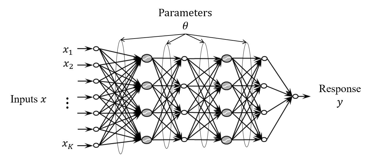
We now have the optimization problem
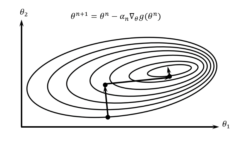
\[\min_{\theta}{g(\theta) = \sum_{n = 1}^{N}\left( y^{n} - f\left( x^{n} \middle| \theta \right) \right)^{2}}. \tag{1.3}\label{eq:mato-1-3}\]We can solve this using a gradient-based search algorithm that looks like:
\[\theta^{n + 1} = \theta^{n} - \alpha_{n}\nabla_{\theta} g(\theta^{n}) \tag{1.4}\label{eq:mato-1-4}\](Note that we use the negative gradient because we are minimizing). You need to talk the students through the process of finding the gradient (and possibly explaining what this is). One key step is finding the stepsize $\alpha_{n}$ which is done by solving the one-dimensional search problem:
\[\alpha_{n} = \arg\max_{\alpha > 0} g(\theta^{n} - \alpha \nabla_{\theta} g\left( \theta^{n} \right)) \tag{1.5}\label{eq:mato-1-5}\]The figure below illustrates the search process.
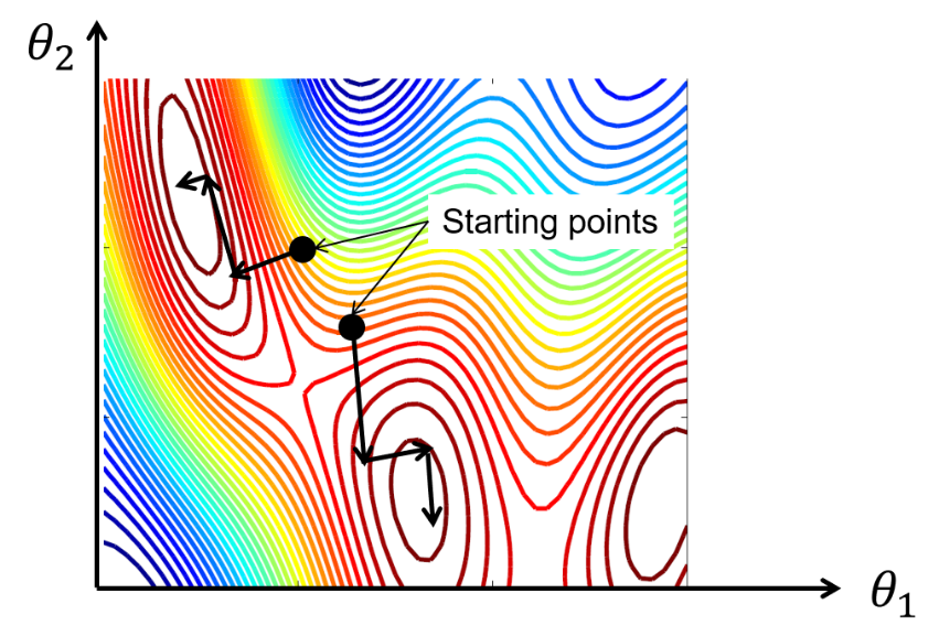
One issue that often arises is that the function $g(\theta)$ may have local minima (illustrated below), which means your gradient algorithm may produce different optima depending on the starting point.
Also – I would note that while we need $n \geq p$ to use the normal equations for our linear model (in Topic 1), we no longer require this for the nonlinear model. We can apply the gradient algorithm for any value of $n$, even if it is smaller (and potentially much smaller) than $p$. Students need to understand that just because the algorithm returns an estimate of the best value of $\theta$, that does not mean that it is guaranteed to be a good value that will work well on future datasets.
You can start by illustrating it using a linear model, and then show how to use it for a nonlinear model. For example, fit a logistic regression to predict demand as a function of price, or probability of winning a bid for placing an ad on Google or Facebook. Then extend to a simple neural network. Be sure to highlight the presence of multiple optima and the need to use multiple starting points. Then, show that you get an answer even when $n < p$, an issue that becomes important with deep neural networks.
This will create a basis for later discussing a well-known issue with neural networks (all students will have heard of this as “AI”) which use models where $p \gg n$. Students will also learn that there is not a unique solution when we optimize parameters for nonlinear models. Finally, I would also make the point that while linear models require $n \geq p$, nonlinear models do not. We can fit a neural network with 100 million parameters with a single datapoint (!).
1.3 Neural networks (optional)
A special kind of nonlinear model is a neural network. Given the visibility of this technology, an instructor may wish to introduce students to the basic idea of a neural network, since the calculations are relatively simple. It is easy to show how to construct a basic neural network, and how to take a vector of inputs and translate it to an output (or set of outputs). Section 3.9.3 of RLSO describes how to compute the output of a neural network through a simple forward pass.
You can then jump to section 5.5 of RLSO if you wish to show how to compute the gradient of a neural network with respect to the weights on each link (these are the tunable parameters). Key to neural networks is that these derivatives are easy to compute. Given the interest in deep neural networks, you can show how these calculations can be done in parallel, which is why chips such as those by Nvidia (which are designed for massively parallel computation, originally for the graphics in video games) are so popular.
I would also point out that there are packages such as TensorFlow that do these calculations very efficiently. However the calculations are performed, the core ideas are the same as what we illustrated using the logistic regression example in section 1.2. Remember – the idea in an introductory course is not to prepare students to actually do research on this topic; it is only to introduce them to important optimization problems and how we go about solving them. For example, the issue of multiple local optimal solutions that we introduced in our section on nonlinear models above is important, since it helps to understand that the “optimal” solution we obtain is not truly optimal, and that small changes in inputs might result in finding a different local solution.
Also – remember that while we require $n \geq p$ in a linear model, we have no such requirement for nonlinear models, including neural networks. We might have a neural network with 100 million parameters, but we will still get a number if we try to train it with just one data point. While this seems silly, it is quite common to fit neural networks where the number of observations (that is, the size of the training dataset) is quite a bit smaller than the number of parameters.
I don’t personally encourage including this material, but it fits very nicely here, and might go a long way to attracting student interest.
1.4 Teaching notes for machine learning
There are some key points that should be brought out in this topic:
- The linear model is a nice opportunity to remind students of some basic linear algebra when deriving the normal equations.
- Be sure to bring out the requirement that $[X^TX]$, where $X$ is the “design matrix” of data, must be invertible, which requires that $n \geq p$. I suggest illustrating with the problem of fitting a line to a single data point, and then to two data points where $x$ is the same for each one.
- The objective functions (equations $\eqref{eq:mato-1-2}$ and $\eqref{eq:mato-1-3}$) look like deterministic optimization problems, but they are not. Fitting a function (linear or nonlinear) to data is actually a stochastic optimization problem which should be written
Here we view $X$, the explanatory variables (also known as independent variables or covariates), and the response $Y = f(X|\theta)$, as random variables. We assume we are given a sample of these variables
\[\left( x^{1},y^{1} \right),\ \left( x^{2},y^{2} \right),\ldots,\left( x^{N},y^{N} \right),\]which we call the training dataset. However, this is just a sample of the random variables $X$ and $Y$, which turns our stochastic optimization problem $\eqref{eq:mato-1-6}$ into a deterministic optimization problem ($\eqref{eq:mato-1-2}$ or $\eqref{eq:mato-1-3}$). We are going to use this technique over and over again in this course to handle virtually any form of uncertainty. The only difference in future applications is that we may need a way of generating our own random sample.
Topic 2: Sequential decision problems I
The vast majority of all decision problems are sequential decision problems. Later, we are going to motivate harder decision problems that use linear, nonlinear and integer programming, but to start we are going to use simpler problems which are still important as well as challenging.
2.1 Introduction to sequential decision problems
Readings: SDAM Chapter 1 (introduction to sequential decision problems).
A sequential decision problem is any problem that consists of the sequence:
decision, information, decision, information, …
where each decision receives a contribution or incurs a cost. Sequential decision problems cover an extremely broad class of optimization problems. Most important is that they cover problems that arise in almost any setting: business, health (all kinds), energy, economics, laboratory experiments, field experiments, …, the list is endless, which means it is possible to illustrate these problems with applications that are suitable to any class.
Decisions are made with methods that we call “policies.” There are two broad strategies for designing policies, and each of these produces two classes, creating four classes of policies:
Strategy 1 – Policy search – This is where we identify a class of functions for making decisions, and then search for the best function that works well over time. The two classes of policies in this strategy are:
- Policy function approximations (PFAs) – These are analytical functions that take what we know to determine what decision to make now. Examples are order-up-to policies for inventory, or buy low, sell high policies in finance.
- Cost function approximations (CFAs) – These are simplified (usually deterministic) optimization models that have been parameterized to work well under uncertainty. We will see CFAs when we introduce optimal learning (Topic 4). We will also see these when we introduce linear, integer and nonlinear programming in topics 7-11.
Strategy 2 – Lookahead approximations – We estimate the value of a decision by combining the immediate cost or reward of a decision plus some approximation of downstream costs and rewards from the initial decision. This strategy can be divided into two classes:
- Value function approximations (VFAs) – Here we find the decision that optimizes the immediate cost or reward plus an approximate value of the state that the decision takes us to. These are the only policies that use Bellman’s equation (Hamilton-Jacobi if you are a controls person).
- Direct lookahead approximations (DLAs) – Finally we optimize the immediate cost or reward plus an estimate of downstream costs or rewards computed by solving an approximate model of the future.
Note that sequential decision problems arise throughout human activities. PFAs are the simplest class and are the most widely used. Most important, these are parameterized functions, just like the parametric models in statistics that we saw in Topic 2.
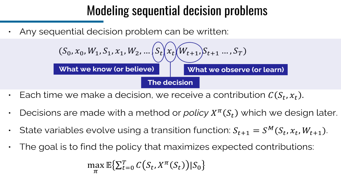
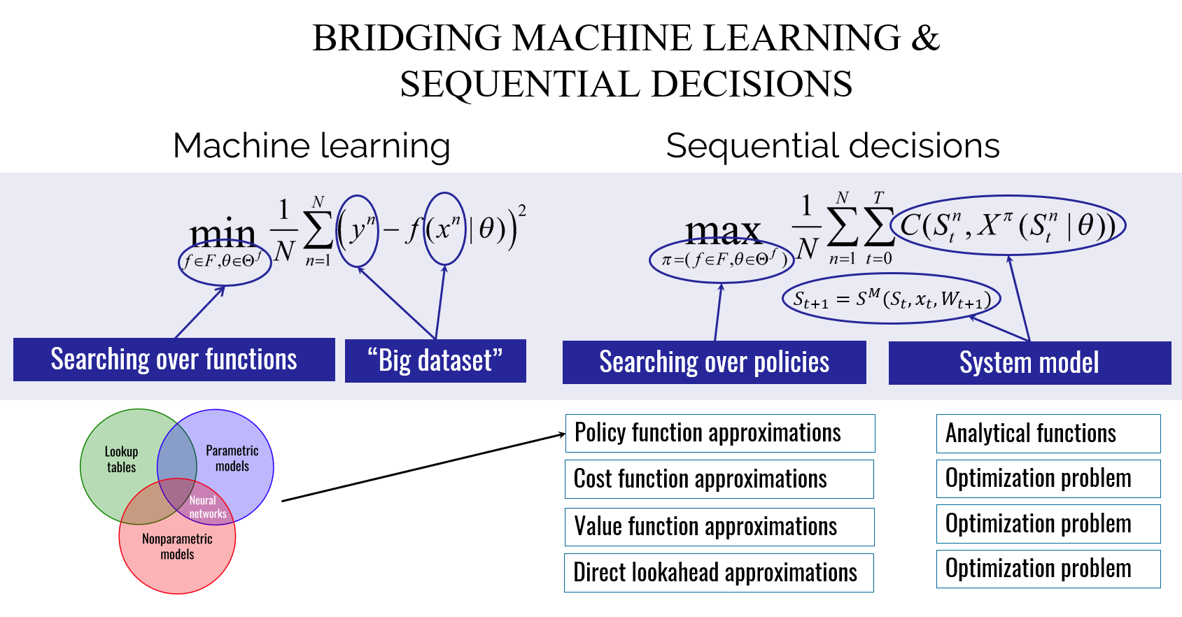
Below is the slide I use to present the elements of a sequential decision problem. It illustrates the notation of states $S_{t}$ (what we know at time t), decisions $x_{t}$ (what decision we choose from a set of feasible decisions), and the exogenous information $W_{t + 1}$ that we learn only after we make the decision $x_{t}$. Decisions are made with a method (policy) that we designate as $X^{\pi}(S_{t}|\theta)$ that often depends on tunable parameters $\theta$. Also shown is the contribution (if we are maximizing) or cost (if minimizing) $C(S_{t},x_{t})$ which may depend on information in the state $S_{t}$ (such as dynamically changing prices or costs) in addition to the decision $x_{t}$. The transition function $S^{M}(S_{t},\ x_{t},\ W_{t + 1})$ gives the updated state $S_{t + 1}$ given the information in $S_{t}$, the decision $x_{t}$, and the exogenous information $W_{t + 1}$.
The next slide (below) is one I use to compare machine learning with sequential decisions. The difference between machine learning and sequential decisions is that with machine learning, you need a training dataset to fit a general-purpose function, whereas sequential decisions (which do not need a training dataset) need a model of the underlying problem (such as the evolution of inventories). It is important to emphasize this difference, since it is often overlooked (especially in discussions of “AI”).
There is a wide range of sequential decision problems that will be familiar to students (unlike linear programs). The challenge is that sequential decision problems involve the arrival of new information, which puts even simple decision problems into a class that has been treated under a wide variety of names, with the most common being “dynamic programs.” This will produce gasps of “oh, that is stochastic optimization…you can’t teach stochastic optimization in an introductory optimization course.” For most faculty, “dynamic programming” means teaching Bellman’s equation.
We are not going to go down that path. First, we observe that both of the machine learning problems in Topics 1 and 2 are forms of stochastic optimization problem. We avoid the complexities that would normally arise by tuning our statistical models used a training dataset that we assumed was given to us.
We are going to follow the same strategy for sequential decision problems, emphasizing three types of policies that are widely used, and which students will typically be familiar with. These are:
- PFAs – These are the simplest policies such as buy low, sell high in finance or order-up-to policies for inventory planning. Note that PFAs include every possible model that might be used in machine learning, which might be anything from a linear model to a deep neural network.
- CFAs – These will be simplified (always deterministic) optimization problems that might involve nothing more than a sort. For more complex problems, we will introduce linear programs, and then show how we can parameterize a linear program to make it work well over time. This powerful idea is widely used in practice but has been completely ignored in the academic literature.
- Deterministic DLAs – Google maps is a nice example of a deterministic DLA, since it plans a path to a destination (which requires looking into the future). For problems where we need to plan into the future, the most widely used strategy is to use a deterministic approximation. We might use tunable parameters to make these perform better over time, but not always.
Below we are going to illustrate some simple sequential decision problems using PFAs, which require tuning parameters. The approach exactly parallels what we did in Topic 1 for machine learning.
2.2 Asset selling
Readings: SDAM Chapter 2.
We are going to start with a simple buy-low, sell-high policy in finance, which offers an important simplification to help us get started: the random information (the price at which we can sell our asset) is drawn from history, allowing us to treat it just as we did the observations $y^{n}$ in our machine learning problems in Topic 1.
We are going to assume that we are given a historical sequence of prices
\[(p_{t - H},p_{t - H + 1},\ldots,p_{t'},\ldots,p_{t})\]where time $t’$ is any point in time in the history where we might sell an asset (assume for simplicity that we can only sell at the end of each day). The price $p_{t}$ would be the most recent price we have available. A nice feature of this problem is that we can assume that the prices are independent of any decisions that we make.
Next imagine that we are going to use the following policy that determines when to buy, sell or hold a single asset
\[X^{\pi_{1}}\left( S_{t} \middle| \theta \right) = \begin{cases} +1 & \text{Sell if } p_{t} > \bar{p}_{t - 1} + \theta_{1} \\ 0 & \text{Hold if } \bar{p}_{t - 1} - \theta_{2} \leq p_{t} \leq \bar{p}_{t - 1} + \theta_{1} \\ -1 & \text{Buy if } p_{t} < \bar{p}_{t - 1} - \theta_{2} \end{cases} \tag{2.1}\label{eq:mato-2-1}\]where
\[\bar{p}_{t} = .5p_{t} + .35p_{t - 1} + 0.15p_{t - 2} \tag{2.2}\label{eq:mato-2-2}\]is a smoothed estimate of prices. The variable $S_{t}$, which is called the “state variable,” captures all the information we know at time t, that we need to make a decision (that is, compute our policy $X^{\pi_{1}}\left( S_{t} \middle| \theta \right)$), as well as any other information we might need. For this problem, the state variable consists of
\[S_{t} = (p_{t},p_{t - 1},p_{t - 2}).\]It is easy to see that our policy $X^{\pi_{1}}\left( S_{t} \middle| \theta \right)$ is one of many possible strategies we could use. This policy has two tunable parameters. To tune the parameters, we need an objective function.
The objective function we would use to perform our tuning would look like
\[F(\theta) = \sum_{t' = t - H}^{t}{X^{\pi}\left( S_{t'} \middle| \theta \right)p_{t'}}. \tag{2.3}\label{eq:mato-2-3}\]Note that our policy depends only on information that we would know at time t, even though we have an entire history of prices $(p_{t - H},p_{t - H + 1},\ldots,p_{t’},\ldots,p_{t})$. This type of tuning is widely used in finance, and is known as “backtesting” since it requires using historical prices to evaluate the policy.
This objective closely parallels the one we used to fit nonlinear models in Topic 1. If we let $\theta_{1} = \theta_{2}$, then we have a one-dimensional problem, which could be easily optimized in a spreadsheet (it is not much harder to do this over two dimensions).
This exercise accomplishes several educational objectives:
- It introduces the idea of a policy for making decisions.
- It uses historical data to represent a sample of outcomes, just as we created a training dataset for machine learning (see Topics 1 and 2).
A different way to perform the tuning is to create a mathematical model of prices, and use this to create a brand new set of prices for each iteration of the algorithm. We do not have to do this for this specific problem, although the tuning would be more robust if we did. However, creating mathematical models of prices is relatively difficult – we would need to capture both the distribution of prices (which is fairly easy) in addition to the correlations of prices over time (this is quite difficult). Working with historical prices avoids these complications.
2.3 Inventory planning
Reading: Section 1.3 of SDAM
Inventory problems are one of the most popular applications of sequential decision problems. This will be a fairly minor variation of the asset selling problem, but it opens the door to an incredibly rich set of applications that arise in supply chain management.
For this topic, we will start with a vanilla inventory problem where we define:
| $R_{t}$ | The amount of inventory at time $t$. |
| $x_{t}$ | The amount of new inventory we order, where we assume it arrives right away. |
| $\hat{D}_{t + 1}$ | The demand for product that arises between $t$ and $t+1$ (and after we make the decision $x_{t}$). |
| $p$ | The unit price at which we sell the product. |
| $c$ | The unit cost of ordering more product. |
The basic equation for updating the inventory $R_{t}$ is given by
\[R_{t + 1} = \max\{0,R_{t} + x_{t} - \hat{D}_{t + 1}\} \tag{2.4}\label{eq:mato-2-4}\]Unlike our asset selling problem, we generally do not get to observe the actual demands $\hat{D}_{t}$, which means we cannot just use a set of observations from history. Instead, we are going to need to generate a set of observations of demands using a random number generator. We are going to take advantage of a standard function built into all computer languages to generate a random number between 0 and 1. For example, in Excel this function is called Rand(). In Python it is called Random.uniform(0,1). We are going to just let the function be represented by $U()$.
If we want a random number $R$ that is uniformly distributed between $a$ and $b$, we use
\[R = a + (b - a)U(). \tag{2.5}\label{eq:mato-2-5}\]Now imagine that we know that on average the demand is $\mu$, where our actual demand $\hat{D}_{t}$ is given by
\[\hat{D}_{t} = \mu + \varepsilon, \tag{2.6}\label{eq:mato-2-6}\]where $\varepsilon$ is a random error term that is uniformly distributed between $-\mu$ and $+\mu$. We can generate random observations of $\varepsilon$ using
\[\varepsilon = -\mu + 2\mu\ U(). \tag{2.7}\label{eq:mato-2-7}\]If we want 100 observations of demands, we need to generate 100 observations of $\varepsilon$.
Now that we have a set of random demands $\hat{D}_{1},\hat{D}_{2},\ldots,\hat{D}_{t},\ldots,\hat{D}_{T}$, we need a method for making decisions. We are going to use a policy known in the literature as an “$(s,S)$” policy where $s$ and $S$ are tunable parameters. We like to use $\theta$ for our tunable parameters, so we are going to replace $s$ and $S$ with $\theta^{\min}$ and $\theta^{\max}$. Our policy is then given by
\[X^{\pi}\left( S_{t} \middle| \theta \right) = \begin{cases} \theta^{\max} - R_{t} & \text{if } R_{t} < \theta^{\min} \\ 0 & \text{otherwise.} \end{cases} \tag{2.8}\label{eq:mato-2-8}\]Our challenge now is to find the best value of $\theta = \left( \theta^{\min},\theta^{\max} \right)$, which we do by optimizing the objective function
\[\max_{\theta} \sum_{t = 0}^{T} \Big( p \cdot \min\big\{ R_{t} + X^{\pi}\left( S_{t} \middle| \theta \right),\ \hat{D}_{t + 1} \big\} - c\, X^{\pi}\left( S_{t} \middle| \theta \right) \Big), \tag{2.9}\label{eq:mato-2-9}\]where the inventory $R_{t}$ evolves according to equation $\eqref{eq:mato-2-4}$.
The optimization problem in $\eqref{eq:mato-2-9}$ can be approached just as we did to optimize our nonlinear model in Topic 1 (equation $\eqref{eq:mato-1-3}$) or the asset selling problem in section 2.2.
2.4 Teaching notes
- We have now seen that optimizing a parameterized policy closely parallels optimizing the parameters of a nonlinear function for machine learning. One difference is that we can generally compute the gradient of the nonlinear function in machine learning, whereas this is typically not true when we are simulating a policy.
- The simplest approach to use right now is to introduce the idea of numerical derivatives.
- There is also a wide range of derivative-free methods, but these should be introduced slowly over the course, depending on the interests of the professor and the backgrounds of the students.
Topic 3: Adaptive optimization – the newsvendor problem
Readings: SDAM Chapter 3
Arguably one of the most widely encountered problems when managing resources is the newsvendor problem, which is a nice illustration of a decision problem involving uncertainty. We will show how to solve this using a simple stochastic gradient algorithm that can be implemented in an online (learn as you go) setting. This is a natural extension of the gradient-based method we used in section 1.2 for optimizing the parameters of a nonlinear statistical model.
In Topic 1, we solved the following machine learning problem
\[\min_{\theta}{\bar{F}\left( x \middle| \theta \right) = \frac{1}{N}\sum_{n = 1}^{N}\left( y^{n} - f\left( x^{n} \middle| \theta \right) \right)^{2}}. \tag{3.1}\label{eq:mato-3-1}\]This is a sampled estimate of the function
\[\min_{\theta}{F\left( x \middle| \theta \right) = \mathbb{E}\left( Y - f(X|\theta) \right)}, \tag{3.2}\label{eq:mato-3-2}\]where “$Y$” is a random variable representing the response given the random input “$X$”, and where
\[\left( x^{1},y^{1} \right),\ \left( x^{2},y^{2} \right),\ldots\ \left( x^{n},y^{n} \right),\ldots\ \left( x^{N},y^{N} \right),\]is a sample of $N$ observations of the variables $(X,Y)$.
The idea of using a sampled estimate to transform a stochastic optimization problem $\eqref{eq:mato-3-2}$ into a deterministic optimization problem $\eqref{eq:mato-3-1}$ is a powerful and widely used strategy when optimizing functions of random variables.
One of the most popular stochastic optimization problems is the newsvendor problem, where we need to choose a quantity $x$ to meet an unknown demand $D$. The challenge is that we have to purchase $x$ units of a product at a unit cost $c$, to meet the demand $D$ receiving a revenue $p$ for each unit sold. The problem is that we cannot sell more than the demand, giving us the objective function
\[\max_{x}{F\left( x \middle| D \right) = p\min\left\{ x,D \right\} - cx}. \tag{3.3}\label{eq:mato-3-3}\]The function $F(x|D)$ assumes we know the demand $D$, but we do not. What we have to do is to find the quantity $x$ that maximizes the expected value of $F(x|D)$ over the random quantity $D$. This would be written
\[\max_{x}{g(x) = \mathbb{E}_{D}F\left( x \middle| D \right) = \mathbb{E}_{D}\left\{ p\min\left\{ x,D \right\} - cx \right\}} \tag{3.4}\label{eq:mato-3-4}\]Imagine that we have a historical dataset of order quantities and demands which we can write out as
\[\left( x^{1},D^{1} \right),\ \left( x^{2},D^{2} \right),\ldots\ \left( x^{n},D^{n} \right),\ldots\ \left( x^{N},D^{N} \right).\]If we have this data, we could solve our problem just as we did our machine learning problem in $\eqref{eq:mato-3-1}$:
\[\max_{x}{\bar{F}(x) = \frac{1}{N}\sum_{n = 1}^{N}\left( p\min\left\{ x,D^{n} \right\} - cx \right)}. \tag{3.5}\label{eq:mato-3-5}\]The problem with this approach is that we never have a set of observations of demands $D^{1},D^{2},\ldots,D^{N}$ because we do not observe demands – we observe what we sell which is the smaller of what we ordered $x^{n}$ and the true demand $D^{n}$. If we order $x^{n} = 6$ and observe sales of 6, it might be that $D^{n} = x^{n}$, but more often it means that $D^{n} > x^{n}$.
There is a simple way to get around this problem. We are going to use a basic gradient search algorithm, but we cannot take the derivative of the function $g(x)$. What we are going to do seems magical (that is, it seems as if we should not be able to do it). We are going to assume that we choose a quantity $x = x^{n}$, and then observe a demand $D^{n + 1}$. Note that we have introduced a subtle shift in how we are indexing $x^{n}$ and the demand $D^{n + 1}$; this way of indexing means that $x^{n}$ depends on $D^{1},\ldots,D^{n}$ but does not depend on $D^{n + 1}$.
After we observe the demand, we now have the deterministic function
\[g\left( x \middle| D^{n + 1} \right) = p\min\left\{ x,D^{n + 1} \right\} - cx. \tag{3.6}\label{eq:mato-3-6}\]Next we are just going to take the derivative of $g\left( x \middle| D^{n + 1} \right)$ with respect to $x$:
\[\nabla g\left( x|D^{n + 1} \right) = \frac{dg\left( x \middle| D^{n + 1} \right)}{dx} = \begin{cases} p - c & \text{if } x \leq D^{n + 1} \\ -c & \text{if } x > D^{n + 1} \end{cases}. \tag{3.7}\label{eq:mato-3-7}\]We now use the same gradient-based search algorithm we first introduced in Topic 1 for nonlinear models:
\[x^{n + 1} = x^{n} + \alpha_{n}\nabla g\left( x|D^{n + 1} \right). \tag{3.8}\label{eq:mato-3-8}\]Unlike our first use of gradient based methods in Topic 1, we can no longer find the stepsize $\alpha_{n}$ by solving a one-dimensional search problem as we did in equation $\eqref{eq:mato-1-5}$. Instead, we are going to use something that is much simpler:
\[\alpha_{n} = \frac{1}{n}. \tag{3.9}\label{eq:mato-3-9}\]Incredibly, we can show that this stepsize rule will produce a sequence of decisions $x^{1},x^{2},\ldots,\ x^{n},$ where
\[\lim_{n \rightarrow \infty}x^{n} \rightarrow x^{*}. \tag{3.10}\label{eq:mato-3-10}\]This means that if we run this algorithm an infinite number of times, it will find the optimal solution! The bad news is that it is possible that the algorithm will be quite slow. A lot of research has gone into finding better stepsize formulas. One way speed up the algorithm is to insert a tunable parameter giving us
\[\alpha_{n}(\theta^{step}) = \frac{\theta^{step}}{\theta^{step} + n - 1}. \tag{3.11}\label{eq:mato-3-11}\]where $\theta^{step}$ is a parameter that has to be tuned. OK, so we have another problem that involves tuning a parameter, but the core idea here is quite simple!
Stochastic gradient algorithms tend to be taught in advanced stochastic optimization classes. However, they are perfectly appropriate for an introductory optimization course, especially for the context of unconstrained problems. Nonnegativity constraints and upper bounds are easy to handle.
Topic 4: Optimal learning – Finding the best treatment
Readings: SDAM Chapter 4
An important class of optimization problems falls under the umbrella of “optimal learning” where the decision involves what to observe, or what experiment to run. From the information gained from the observation (or experiment), we then use our beliefs to make a choice about a choice of design, or product, or price.
There is an endless array of optimal learning problems – a sample might include:
- Medical treatments (choice of drug, dosage)
- Which product to advertise on a website
- Which supplier to use to supply materials or components
- Which schools to visit to interview for employees
- What price to charge for a product (from a set of prices)
- Who should be starters on a basketball team
- Which path to take through a congested network to get to work
- Which product to recommend on a webpage to attract the most clicks
- Which of several webpage designs to use to maximize traffic
- …(this is a very long list)
In this section we will use the context of finding the best medical treatment for a patient.
Learning the best of a set of “treatments” is widely known as a “multiarmed bandit problem” which is a mathematically rich (and computationally complex) problem. However, the approach we are going to use here is quite simple and very popular at companies like Google and Facebook for optimizing ads (students should resonate with this). In the process, we are also going to introduce a new class of policy that is going to open the door to a much more complex class of problems. These policies are known as “cost function approximations” (or CFAs).
We are going to start with a policy called “interval estimation” that helps us choose the best treatment $x \in X = { x_{1},\ldots,x_{K}}$. Let $\bar{\mu}_{x}^{n}$ be our estimate of the effectiveness of treatment $x$ after we have performed $n$ experiments using any of the choices. Then let $\bar{\sigma}_{x}^{n}$ be the standard deviation of $\bar{\mu}_{x}^{n}$ (remind students how to do the standard deviation of a mean, and how it goes to zero as $n \rightarrow \infty$).
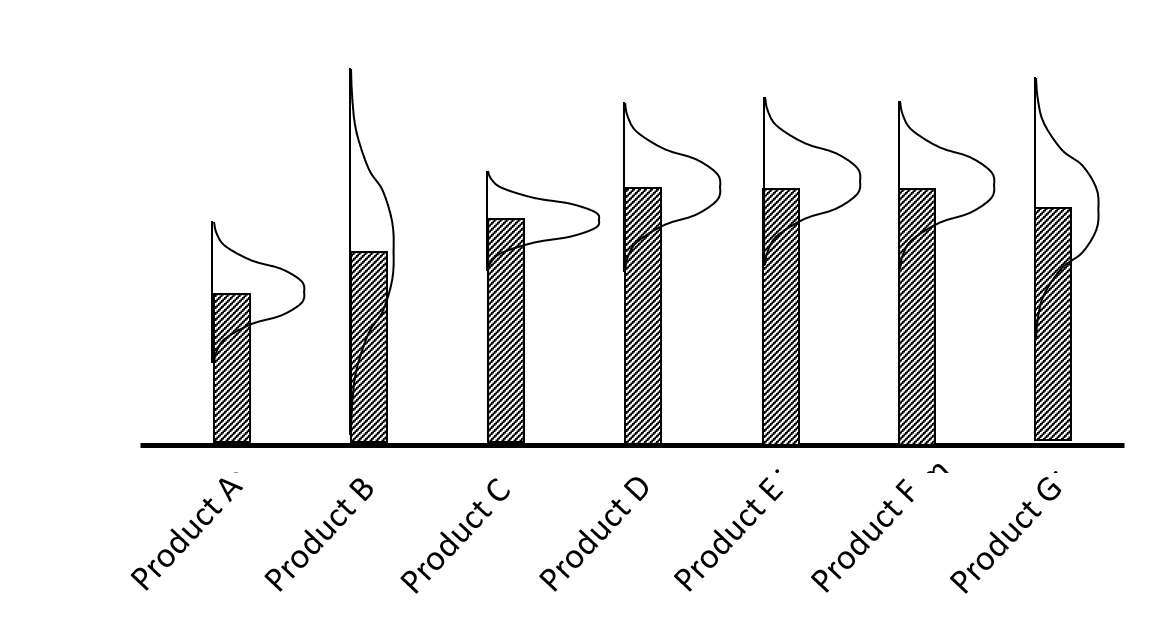
After $n$ experiments, our beliefs might look like those shown in the figure above – this might represent the potential sales of different products, but there are many settings where this applies. We represent our beliefs using the belief state variable $B^{n} = \left( \bar{\mu}_{x}^{n},\bar{\sigma}_{x}^{n} \right)_{x \in X}$ to capture our beliefs about the performance of each choice $x$. For this problem, the state variable $S^{n} = B^{n}$ equals the belief state, but there are problems where we may have information other than the belief state (such as the budget remaining to run experiments). For now, we are just going to limit the state variable to the belief state.
The interval estimation policy is given by:
\[X^{IE}\left( S^{n} \middle| \theta^{IE} \right) = \arg\max_{x \in X}\left( \bar{\mu}_{x}^{n} + \theta^{IE}\bar{\sigma}_{x}^{n} \right) \tag{4.1}\label{eq:mato-4-1}\]where $x^{n} = X^{IE}\left( S^{n} \middle| \theta^{IE} \right)$ is the design we are going to choose for the $n + 1^{\text{st}}$ experiment, which produces an observation $W^{n + 1}$.
With our inventory problem, we updated our state variable (the inventory) using the inventory equation $\eqref{eq:mato-2-4}$. With a learning problem, we have to update our beliefs, which we are going to do using some simple recursions. Assume that we observe performance $W_{x}^{n + 1}$ when we test choice $x = x^{n}$. First, we are going to replace the variances $\left( \bar{\sigma}_{x}^{n} \right)^{2}$ with their inverses which we call the precision given by
\[\beta_{x}^{n} = \frac{1}{\left( \bar{\sigma}_{x}^{n} \right)^{2}}. \tag{4.2}\label{eq:mato-4-2}\]We are also going to assume that when we observe the results of an experiment which we represent by $W_{x}^{n + 1}$ that this experiment is random with a known variance $\sigma_{W}^{2}$ and precision
\[\beta^{W} = \frac{1}{\sigma_{W}^{2}}. \tag{4.3}\label{eq:mato-4-3}\]We can use the precision to write the updating equations for the means and precisions using
\[\bar{\mu}_{x}^{n + 1} = \frac{\beta_{x}^{n}\bar{\mu}_{x}^{n} + \beta^{W}W_{x}^{n + 1}}{\beta_{x}^{n} + \beta^{W}}, \tag{4.4}\label{eq:mato-4-4}\] \[\beta_{x}^{n + 1} = \beta_{x}^{n} + \beta^{W}. \tag{4.5}\label{eq:mato-4-5}\]Equations $\eqref{eq:mato-4-4}$ and $\eqref{eq:mato-4-5}$ represent the transition equations $S^{n + 1} = S^{M}(S^{n},x^{n},W^{n + 1})$ for this problem.
An important feature of our interval estimation policy $\eqref{eq:mato-4-1}$ is that imbedded in the policy is an optimization problem. Here the optimization (given by the “argmax”) requires nothing more than a simple sort over the alternatives to find one with the best value of $\bar{\mu}_{x}^{n} + \theta^{IE}\bar{\sigma}_{x}^{n}$. Later, we are going to replace this with more sophisticated optimization problems. For example, in Topic 5, our imbedded optimization problem will be a shortest path problem. In Topic 7 the imbedded optimization problem will be a linear program, which we see again in Topic 8 when we are dynamically planning energy storage. In Topic 10 the imbedded optimization problem will be an integer program, and in Topic 11 (section 11.2) the imbedded optimization problem will be a nonlinear programming problem.
The interval estimation policy is very easy to implement, but it is important not to overlook the need to tune the parameter $\theta^{IE}$. One way to do this is to run a simulation where we assume that we know the true performance of each alternative $x$ which we denote by $\mu_{x}$. If we choose to test alternative $x$, we cannot observe $\mu_{x}$ perfectly – instead, we can only perform a noisy observation where we add a noise term $\varepsilon$. This means that the observed performance of $x = x^{n}$ would be given by
\[W_{x}^{n + 1} = \mu_{x^{n}} + \varepsilon. \tag{4.6}\label{eq:mato-4-6}\]We can use the methods we presented for the inventory planning problem (see equations $\eqref{eq:mato-2-5}$-$\eqref{eq:mato-2-7}$) to generate random observations of $\varepsilon$. Now, create $N$ (say, $N$=100) observations of $W_{x}^{n}$ for each alternative $x$ and store these. Now, simulate our interval estimation policy $X^{IE}(S^{n}|\theta^{IE})$ which we evaluate using
\[F(\theta) = \sum_{n = 1}^{N}W_{x^{n}}^{n} \tag{4.7}\label{eq:mato-4-7}\]where $x^{n} = X^{IE}(S^{n}|\theta^{IE})$ and where the state variable $S^{n}$ is updated using equations $\eqref{eq:mato-4-4}$ and $\eqref{eq:mato-4-5}$. Note that we have written $\eqref{eq:mato-4-7}$ as if we are running a single simulation. We can do this, but it will be noisy. Instead of pre-generating the outcomes of $W_{x}^{n}$ and using these in the simulation of the policy, it makes more sense to generate them on the fly (this is very fast using any programming language such as Python). Now compute the sum in $\eqref{eq:mato-4-7}$, say, 1000 times and take an average. Finally, repeat this for a discrete set of values of $\theta$ such as 0, 0.1, 0.2, …, 4.0 and choose the value of $\theta^{IE}$ that works the best.
Topic 5: Shortest path problems
We are going to use shortest path problems as our first small step into a nontrivial decision problem. While this is technically a linear program, we will be able to demonstrate a simple algorithm based on Bellman’s equation that everyone can understand. Shortest path problems also provide a nice visual setting to later illustrate the idea of a basis and pivoting (but this is for later).
We are going to first present the static shortest path problem, and then transition to using this in a dynamic setting as would occur when you are driving from one location to the next while your navigation system is responding to new information. It is in the dynamic setting that we will see that a shortest path problem is a form of policy (specifically a direct lookahead policy, or DLA) that can, if we like, be parameterized to help deal with uncertainty.
5.1 Static shortest paths
This lecture is based on chapter 5 of SDAM.
This will be our first peek at a specialized linear program that we will solve using a classical Bellman iteration. This is very simple in the context of a network problem since the “state” variable is just the node where the traveler is located.
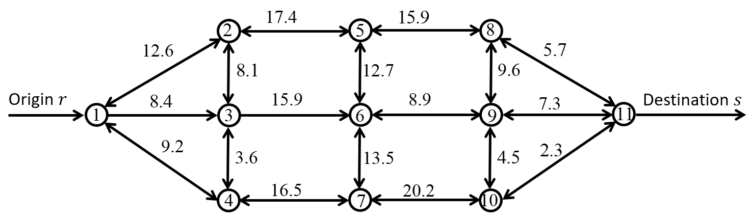
Assume we are trying to find the shortest path from an origin at node 1 to a destination at node 11. Let $v_{i}$ be the minimum cost to get from node $i$ to the destination node 11. We are going to initialize $v_{11} = 0$, and set $v_{i}$ equal to some large number for all other nodes $i \neq 11$.
Let $N_{i}^{+}$ be the set of nodes we can reach from node $i$.
A simple (but not very efficient) algorithm for finding the shortest path from each node to node 11 would be to repeatedly compute for every node $i$
\[v_{i} = \min_{j \in N_{i}^{+}}{(c_{ij} + v_{j})}. \tag{5.1}\label{eq:mato-5-1}\]The idea is to repeatedly loop over all nodes $i$ and compute $\eqref{eq:mato-5-1}$ until none of the node values change. We can store the optimal solution by letting
\[x_{ij}^{*} = \begin{cases} 1 & \text{if } j = \underset{k \in N_{i}^{+}}{\arg\min}{(c_{ik} + v_{k})} \\ 0 & \text{otherwise} \end{cases} \tag{5.2}\label{eq:mato-5-2}\]Equation $\eqref{eq:mato-5-1}$ is known as Bellman’s equation and is very popular in the academic literature for solving a wide range of sequential decision problems. In practice, it only works for a very small subset of problems, but this happens to be one where it works very well (although commercial algorithms use a lot of shortcuts).
We can trace the shortest path by starting at node 11 and then traversing from any node $i$ to the node $j$ where $x_{ij}^{*} = 1$.
5.2 Dynamic shortest paths
Readings: SDAM Chapter 6
Here we introduce the problem faced by Google maps. We have to route a traveler through a network where new information is arriving over time. Imagine that time steps forward one increment each time we traverse a link. When the traveler arrives at node $i$ at time $t$, Google receives updated estimates of travel times and recomputes the shortest path. This is a dynamic system where the “state” now includes two pieces of information: the node where the traveler is located (node $i$), and the updated estimates of the travel times over the entire network.
To keep the notation simple, assume that we get updates of estimated travel times at each time period, although in reality we only need to update the travel times each time a traveler arrives at a node and has to make a decision. Now, instead of a fixed cost $c_{ij}$, we have costs that are updated and depend on time $t$, so we define $c_{tij}$ as the estimated travel time on each link $(i,j)$ given the information we have at time $t$.
We then solve the same static shortest path problem we did above, but instead we are using the updated costs $c_{tij}$, and obtain the updated path $x_{tij}^{*}$. We are not going to implement the entire shortest path – instead, if we are at some node $i$ at time $t$, we are going to choose to go to node $j$ if $x_{tij}^{*} = 1$.
We can write our shortest path problem at time $t$ using our vocabulary of policies. At time $t$, our state variable $S_{t}$ captures what we know, which includes the node $i_{t}$ where we are located, and the current estimates of all the link costs which we can write as $c_{t} = (c_{tij})$ for all links $(i,j)$ in the network.
So we would write our state variable as
\[S_{t} = \left( i_{t},c_{t} \right).\]Our policy is to solve the static shortest path problem using our updated vector of costs $c_{t}$, but the policy only returns what the traveler should do at time $t$, which we can write as
\[X_{t}^{\pi}\left( S_{t} \right) = x_{i_{t},j}^{*}.\]This means that $X_{t}^{\pi}\left( S_{t} \right)$ is a vector of 0’s with a 1 in the entry corresponding to $x_{i_{t},j_{t}}^{*} = 1$. We will let
\[X_{t i_{t},j}^{\pi}\left( S_{t} \right) = \begin{cases} 1 & \text{if } j = j_{t} \\ 0 & \text{otherwise} \end{cases}\]Let’s introduce a twist. Imagine that we have a goal of reaching our destination by a particular time, and while the shortest path suggests that we will arrive in time, we recognize that there is uncertainty in the travel times. The costs (times) $c_{tij}$ are just the estimated means from the sampled observations we have from watching individual travelers. Instead of using an average, what if we use the 80th percentile, or the 90th percent, or the 50th? These are easy to compute from the raw data.
Let $\theta^{pctile}$ be the percentile of the travel time for a link, and let $c_{tij}\left( \theta^{pctile} \right)$ be the travel time corresponding to the $\theta^{pctile}$ of the travel times.
Now we use $c_{tij}\left( \theta^{pctile} \right)$ for the travel times (instead of the means $c_{tij}$). We would then write our policy as $X_{t}^{\pi}\left( S_{t}|\theta^{pctile} \right)$ to express the dependence on $\theta^{pctile}$. The performance of the policy $X_{t}^{\pi}\left( S_{t}|\theta^{pctile} \right)$ depends on both the actual travel time, but also how late the traveler is for their appointment. Typically we would add a penalty $\theta^{late}$ times how late the traveler is.
Now we have another tuning problem just like we saw with PFAs (Topic 2), and solved using the same methods we saw in Topic 1. To evaluate our policy, let $\hat{c}_{tij}^{n}$ be the sample realization of the actual time to traverse link $(ij)$ that we reach at time $t$. These samples are not used to plan a path – they are only used to evaluate the policy for making decisions. We can generate $\hat{c}_{tij}^{n}$ using the Monte Carlo simulation methods we introduced in section 2.3.
Next let $\hat{F}^{n}(\theta)$ be the actual travel time over the entire path for the $n^{\text{th}}$ trial, using costs $\hat{c}_{tij}^{n}$:
\[\hat{F}^{n}(\theta) = \sum_{t = 1}^{T}{\sum_{ij}{X_{tij}^{\pi}(S_{t}|\theta)\hat{c}_{tij}^{n}}}.\]$\hat{F}^{n}(\theta)$ is the actual travel time we experience in our $n^{\text{th}}$ trip following policy $X_{t}^{\pi}(S_{t}|\theta)$ while experiencing link costs $\hat{c}_{tij}^{n}$. Let’s say that we have to finish the trip in time $\tau$ to arrive in time for our appointment. Let $\eta$ be the penalty per unit time for being late.
The total cost (time plus late penalty) for the $n^{\text{th}}$ trip is then
\[\hat{C}^{n}(\theta) = \hat{F}^{n}(\theta) + \eta\max\left\{ 0,\hat{F}^{n}(\theta) - \tau \right\}. \tag{5.3}\label{eq:mato-5-3}\]We can then write the performance of our policy by averaging over $N$ as
\[\bar{C}^{\pi}(\theta) = \frac{1}{N}\sum_{n = 1}^{N}{\hat{C}^{n}(\theta)}.\]We now have another instance of needing to tune the parameter of a policy.
This lecture is setting the stage for parameterizing linear programs. When we present linear programs in Topic 7, we are going to start by presenting a basic static, deterministic linear program (just as we did with our initial shortest path problem), and then transition to recognizing that the linear program we chose is typically solved repeatedly over time, just as we have done above with our shortest path problem.
Topic 6 – General concepts
Up to now we have been approaching problems in what might appear an ad hoc manner. Actually our problems have been carefully chosen to illustrate some important dimensions of modeling and solving different types of decision problems.
Below we are going to step back and talk more generally about modeling, designing policies, and evaluating policies.
So far we have seen two types of optimization problems:
- Static problems (the machine learning problems in Topic 1, and the shortest path problem in Topic 5, section 5.1).
- Sequential decision problems (Topics 2, 3 and 4, and the dynamic shortest path problem in Topic 5, section 5.2).
Below we are going to provide modeling frameworks for each of these problems.
6.1 Modeling static optimization problems
For our machine learning problems, we faced the problem of minimizing a nonlinear function (the sum of squares of errors) of a set of tunable coefficients $\theta$. If we let
\[F(\theta) = \sum_{n = 1}^{N}{\left( y^{n} - f\left( x^{n} \middle| \theta \right) \right)^{2}}, \tag{6.1}\label{eq:mato-6-1}\]then we can write our optimization problem as
\[\min_{\theta}{F(\theta)}. \tag{6.2}\label{eq:mato-6-2}\]We refer to $F(\theta)$ as our objective function. The standard form that we might use would be to replace $\theta$ with $x$ which is our standard notation for a decision variable, and let $C(x)$ be a generic “cost” function (assuming we are minimizing, which is what is standard in deterministic optimization). Our problem would then be written
\[\min_{x}{C(x)}. \tag{6.3}\label{eq:mato-6-3}\]We can use this style for our shortest path problem, where $x = (x_{ij})$ is the vector of flows over the network. We would let
\[x_{ij} = \begin{cases} 1 & \text{if link } (i,j) \text{ is in the shortest path tree to the destination.} \\ 0 & \text{otherwise} \end{cases}\]We would then write our objective function as
\[C(x) = \sum_{i,j}{c_{ij}x_{ij}}, \tag{6.4}\label{eq:mato-6-4}\]where $c_{ij}$ is the cost of traversing link (i,j). The problem with this formulation is that the optimal solution is $C(x) = 0$ since we would just set $x_{ij} = 0$. We need to introduce constraints so that we guarantee that our optimal solution returns a shortest path from the origin to the destination. We do this by introducing constraints which would be written
\[\sum_{j}x_{ij} - \sum_{i}{x_{ij}} = 0 \quad \text{for } i,\ j \neq \text{origin or destination}, \tag{6.5}\label{eq:mato-6-5}\] \[\sum_{j}x_{ij} - \sum_{i}{x_{ij}} = 1 \quad \text{for } i = \text{origin}, \tag{6.6}\label{eq:mato-6-6}\] \[\sum_{j}x_{ij} - \sum_{i}{x_{ij}} = -1 \quad \text{for } i = \text{destination}. \tag{6.7}\label{eq:mato-6-7}\]We then typically impose the requirement that $x_{ij}$ cannot be negative by writing
\[x_{ij} \geq 0. \tag{6.8}\label{eq:mato-6-8}\]We often want to include upper bounds $u_{ij}$. In our shortest path problem, equations $\eqref{eq:mato-6-5}$-$\eqref{eq:mato-6-7}$ would allow a solution where $x_{ij} > 1$ implying a path that is running in circles (which is clearly not a good idea). If we want upper bounds, we would then write
\[x_{ij} \leq u_{ij}. \tag{6.9}\label{eq:mato-6-9}\]Equations $\eqref{eq:mato-6-5}$–$\eqref{eq:mato-6-7}$ can be written in matrix form
\[Ax = b \tag{6.10}\label{eq:mato-6-10}\]by suitably constructing the matrix $A$ and the vector $b$. By doing this, we can now write our optimization problem in the form
\[\min_{x} C(x) = \sum_{ij}{c_{ij}x_{ij}} = c^{T}x, \tag{6.11}\label{eq:mato-6-11}\]subject to the constraints
\[Ax = b \tag{6.12}\label{eq:mato-6-12}\] \[x \leq u \tag{6.13}\label{eq:mato-6-13}\] \[x \geq 0 \tag{6.14}\label{eq:mato-6-14}\]Equations $\eqref{eq:mato-6-11}$-$\eqref{eq:mato-6-14}$ are a fairly standard way of writing a static optimization problem. What is most important about this framework is that it is a language for thinking about a very large class of decision problems.
An important dimension of modeling optimization problems is the use of constraints such as $\eqref{eq:mato-6-12}$–$\eqref{eq:mato-6-14}$. We first saw constraints in our shortest path problem, but these were enforced by the concept of finding a path. The optimization problems in Topics 1 and 2 were unconstrained. Linear programs (which we introduce in Topic 7) are meaningless without constraints. In fact, we are going to see that expressing problem characteristics through constraints is an art form that is a necessary skill for people who want to use linear programs.
Constraints represent a major feature of static optimization problems. They come in a number of flavors:
- Unconstrained problems, which we saw in Topic 1 for machine learning.
- Upper and lower bounds (also known as “box” constraints), such as $\eqref{eq:mato-6-13}$ and $\eqref{eq:mato-6-14}$.
- General linear constraints such as $\eqref{eq:mato-6-12}$. With some creativity, we can handle a wide range of constrained problems using linear constraints. For our network problem, linear constraints are natural, but later (in Topic 10, section 10.3) we are going to need some creativity to express constraints using linear equations.
- Nonlinear constraints – An example might be $x_{i}\left( 1 - x_{j} \right) = 0$. We do not deal with nonlinear constraints in this course.
Easily the most widely used algorithmic search strategy depends on gradients. The simplest search algorithms are gradient-based, as we saw in section 1.2 for optimizing the parameters of a nonlinear machine learning model, and again in topic 3 for our newsvendor problem. In Topic 7, we are going to see how to use a gradient-based algorithm in the presence of linear constraints using a method that is widely known as the simplex algorithm.
The literature on optimization problems is incredibly rich, but often ignores that an optimization problem is just solving a decision problem at one point in time, whereas the real application involves decisions that are made sequentially over time.
6.2 Modeling sequential decision problems
Modeling any sequential decision problem starts by answering three questions:
- What are the performance metrics?
- What types of decisions are being made (and for larger problems, who makes each type of decision)?
- What are the sources of uncertainty?
The answers to these three questions lay the foundation for building our model.
Any model of a sequential decision problem can be broken down into five components:
State variables $S_{t}$. A "state variable" $S_{t}$ is all the information we need to model the system from time $t$ onward. In other words, the state variable can be viewed as the "state of information" or, more precisely, the "state of knowledge," capturing everything we know or believe that we need to a) compute the objective function (e.g. changing prices and costs), b) make a decision, which means the information needed to represent the available set of actions (e.g. what product to choose among those that are available) or the constraints that determine the feasibility of $x$, and c) any other information needed to model the evolution of information in (a) or (b) (see the "transition function" below).
It is useful to distinguish between the initial state $S_{0}$ that might include static information that never changes (such as the maximum speed of a truck), from the dynamic state variables $S_{t},\ t > 0$ which includes information that is changing over time such as the location of a vehicle moving over a network, the amount of inventory being held, or the evolving prices of an asset.
State variables come in three flavors:
- $R_{t}$ = Vector of physical and financial resources (people, product, equipment, facilities). This can be inventories, or the location of a person or piece of equipment that is moving around. It can also be the amount of cash on hand, investments of different kinds, loans, ...
- $I_{t}$ = Other information about the system not included in $R_{t}$ such as prices, weather, market conditions.
- $B_{t}$ = Beliefs about quantities and parameters that are not known perfectly. This could be the mean and variance of a normal distribution, a vector of probabilities of discrete values of parameters such as a cost or constraint (we first saw belief state variables in Topic 4).
There is tremendous (and surprising) confusion about state variables in the academic literature. There are entire fields (Markov decision processes, reinforcement learning) that never even define a state variable. For a more in-depth discussion see the webpage https://tinyurl.com/onstatevariables/.
Decision variables $x_{t}$. These are the variables that we are controlling. We distinguish between initial decisions $x_{0}$ which are made once (called design decisions), versus $x_{t},\ t > 0$ which are made over time (called control decisions). We represent the feasible decisions by creating a set $X_{t}$ that can be a feasible set of actions (e.g. what link to traverse, which person to hire) or the feasible region defined by constraints such as $\eqref{eq:mato-6-12}$-$\eqref{eq:mato-6-14}$. Finally, we introduce a function $X^{\pi}\left( S_{t} \middle| \theta \right)$, which we call a *policy*, which determines how we make a decision from the information available in the state variable $S_{t}$. Our policies usually depend on tunable parameters $\theta$ (but not always). Most important: *we will determine the policy later!*
Exogenous information $W_{t + 1}$. This is information that we did not know at time $t$, but which became available by time $t+1$ when we have to determine the decision $x_{t + 1}$. In our examples above, the information $W_{1},\ldots,W_{t},\ldots,W_{T}$ is generated in advance, either from history (as we did with the asset selling example) or from Monte Carlo simulation, as we did in the inventory planning example. Although we created this information in advance, we never made a decision $x_{t}$ using the information in $W_{t + 1}$ or later.
Up to now, we have generated a single random sequence of the sequence of observations $W_{1},\ldots,W_{t},\ldots,W_{T}$, which we then used just as we used the training data in our machine learning problems in Topic 1. However, there are settings where $W_{t + 1}$ depends on the state variable $S_{t}$, or the decision $x_{t}$, or both. We can still use a sample of the sequence $W_{1},\ldots,W_{t},\ldots,W_{T}$, but we cannot generate it in advance. Instead, we have to generate it as the system evolves.
Sometimes (in fact, frequently) we want to explicitly capture that there may be more than one sequence of exogenous information. Imagine that we are generating the demands for our inventory problem. Instead of generating one sample, we generate 10 as shown below. Following standard practice from the modeling literature, we let the Greek letter $\omega$ ("omega"), index the sample paths. So, if we generate 10 samples of the demands, $\omega$ would range from 1 to 10.
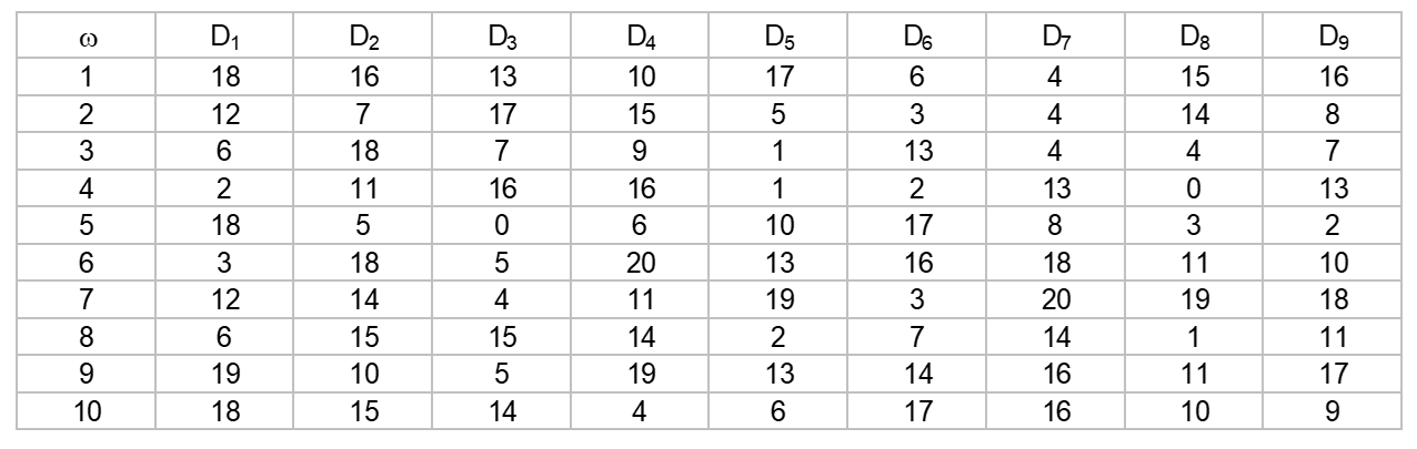
To indicate a particular realization of $W_{t}$, we would write $W_{t}(\omega)$ (if we are using demands $D_{t}$, we would write $D_{t}(\omega)$). We can use this notation to compute, say, the average demand at time $t$ using
\[\bar{D}_{t} = \frac{1}{10}\sum_{\omega = 1}^{10}{D_{t}(\omega)} \tag{6.15}\label{eq:mato-6-15}\]Transition function. This is the function that describes how the information in the state variable evolves over time. We write this function using
$$S_{t + 1} = S^{M}\left( S_{t},x_{t},W_{t + 1} \right). \tag{6.16}\label{eq:mato-6-16}$$
In other words, given what we know (or believe) which is captured in $S_{t}$, the decision we made $x_{t}$, and the new information that arrived from outside the system (which is not known at time $t$), given by $W_{t + 1}$, the transition function returns the updated state variable $S_{t + 1}$. The notation $S^{M}(\cdot)$ stands for "state transition model" (or if you like, "system model").
A transition function can be a single equation such as the inventory equation $\eqref{eq:mato-2-4}$ for our inventory planning problem. However, for complex systems (supply chains, trucking companies, energy systems, health systems) the transition function may require many thousands of lines of code.
Objective function. With deterministic optimization, objective functions are very straightforward, typically summing costs that are minimized, or it might be some performance metric to be maximized.
With sequential decision problems, objective functions can come in different styles. We start by assuming that we are maximizing the cumulative contribution (or reward) over time, as we did in the problems in Topic 2. Let's start by writing the contribution in each time period as $C(S_{t},x_{t})$, the contribution from decision $x_{t}$ made at time $t$, using the information in $S_{t}$ such as a dynamically varying cost or price, such as the price $p_{t}$ in our asset selling problem.
We may write the contribution using $C(S_{t},X^{\pi}\left( S_{t}|\theta \right))$ to reflect the dependence on the policy, since $x_{t} = X^{\pi}(S_{t}|\theta)$.
Now imagine that we have created in advance a random sample of the information sequence $W_{1},\ldots,W_{T}$ as we did in our asset selling example or the inventory planning example. Our objective function would then be written
$$F(\theta) \approx \sum_{t = 0}^{T}{C(S_{t},X^{\pi}\left( S_{t} \middle| \theta \right))} \tag{6.17}\label{eq:mato-6-17}$$
where the transition function $S_{t + 1} = S^{M}\left( S_{t},\ x_{t} = X^{\pi}\left( S_{t} \middle| \theta \right),W_{t + 1} \right)$ is computed with our sampled set of observations $W_{1},\ldots,W_{T}$.
If we wish to use more than one sample of $W_{1},\ldots,W_{T}$, we can assume we have a set $W_{t}(\omega)$ for $\omega = \{\omega^{1},\ldots,\omega^{n},\ldots,\omega^{N}\}$. Now we would model our transition function by reflecting the dependence on the sample $\omega$ which we can write using
$$S_{t + 1}(\omega) = S^{M}\left( S_{t}(\omega),\ x_{t}(\omega) = X^{\pi}\left( S_{t}(\omega) \middle| \theta \right),W_{t + 1}(\omega) \right). \tag{6.18}\label{eq:mato-6-18}$$
We then calculate an estimate of our objective function using
$$F(\theta) \approx \frac{1}{N}\sum_{n = 1}^{N}{\sum_{t = 0}^{T}{C(S_{t}(\omega^{n}),X^{\pi}\left( S_{t}(\omega^{n}) \middle| \theta \right))}} \tag{6.19}\label{eq:mato-6-19}$$
Here we are just running $N$ simulations and taking an average. However we compute the objective function, our optimization problem is then written
$$\min_{\theta}{F(\theta)} \tag{6.20}\label{eq:mato-6-20}$$
Instead of listing constraints as we did in our static objective function (these are built into the design of our policy $X^{\pi}(S_{t}|\theta)$), we would follow the statement of the objective in $\eqref{eq:mato-6-20}$ with the transition function $\eqref{eq:mato-6-16}$ and the information given to the model in the form of the initial state $S_{0}$ and the information $W_{1},\ldots,W_{T}$.
We see that modeling a sequential decision problem is much richer than a static optimization model, but it is roughly a mathematical statement of the simulations that we have already illustrated in Topic 2.
Our modeling framework can be used to model any sequential decision problem, although there are other choices for the objective function. Next we are going to turn to the issue of designing policies, which is a little richer than we have indicated above.
6.3 Designing policies
Above, we wrote our policy as $X^{\pi}(S_{t}|\theta)$ which seems to imply that we already have some functional form for the policy, and then have to tune the parameters $\theta$. However, just as we have to choose between different models in machine learning (such as the linear and nonlinear models we saw in Topic 1), we also have to choose among different functional forms for policies. However, the set of choices becomes much broader.
We can divide all the different types of policies into four classes which cover every possible method for making decisions. These are organized into two broad strategies as follows:
Strategy I: Policy Search. This strategy searches over parameterized functions to identify the ones that work best over time. These come in two classes:
Policy function approximations (PFAs). Analytical functions that map the information in the state variable directly to a decision. Some examples are:
- Buy low, sell high policies in finance -- see asset selling in Topic 2.
- Order-up-to policies for inventories: if the inventory is below $\theta^{\min}$ order up to $\theta^{\max}$ and we then have to tune $\theta = \left( \theta^{\min},\theta^{\max} \right)$ -- see inventory planning in Topic 2.
Linear decision rules are special problems where we can write a policy as:
$$X^{\pi}\left( S_{t} \middle| \theta \right) = \sum_{g \in G}{\theta_{g}\phi_{g}\left( S_{t} \right)}.$$
- A PFA can be any lookup table, parametric function (linear or nonlinear including neural networks) or nonparametric function.
We note that PFAs include every possible functional form that we might use in machine learning.
Cost function approximations (CFAs). A parameterized optimization problem that is typically a deterministic approximation, in which parameters have been introduced to make it work well under uncertainty. CFAs are widely used in industry in an ad-hoc way, but have not been formally studied in the research literature. Some examples include:
- Solving the shortest path over a network with random link times, but using the $\theta$-percentile of the travel times (instead of the mean) -- see Dynamic shortest paths in Topic 5.
- Scheduling aircraft using an integer program, while inserting slack in the schedule to account for weather delays.
- Scheduling nurses but limiting their time to 32 hours per week to provide slack in case emergencies arise.
Strategy II: Lookahead approximations. These policies identify good decisions by optimizing across the current cost or contribution plus an approximation of the effect of a decision now on the future. Again, these come in two classes:
Value function approximations (VFAs). Policies based on VFAs cover all methods based on Bellman's equation, which approximates the downstream value of landing in a state. This approach has attracted tremendous attention under names such as approximate dynamic programming, adaptive dynamic programming, neurodynamic programming, and most commonly today, reinforcement learning. We illustrate Bellman's equation in Static shortest paths (Topic 5, section 5.1), but here the value functions are exact, since we take advantage that our "state" variable is simply which node where the traveler is located.
We can formulate virtually any sequential decision problem using Bellman's equation, but the vast majority cannot be solved exactly. There is by now a substantial literature for estimating value functions approximately, although this approach is more popular in the academic literature rather than used in practice. An in-depth investigation of this strategy is beyond the scope of this course.
Direct lookahead approximations (DLAs). This is where we explicitly plan into the future to help make a decision now. DLAs can be split into two subclasses:
Deterministic DLAs are when we ignore uncertainty to create a deterministic lookahead model, a strategy that is often called a rolling (or receding) horizon procedure, or model predictive control. We do this in Dynamic Shortest Paths (section 5.2).
It is possible to parameterize the lookahead to help make it more robust to uncertainty, producing a hybrid CFA/DLA, as we do in section 5.2.
- Stochastic DLAs create an approximate stochastic lookahead model, typically using sampled approximations of random outcomes. This covers stochastic programming (with scenario trees), robust optimization and approximate dynamic programming, which can be used to solve a simplified stochastic lookahead. This policy is beyond the scope of this course.
These four (meta)classes of policies are universal – they include any method proposed in the research literature or used in practice. None of these methods is a panacea – depending on the specific characteristics of a problem, any one of these may work best. However, some are more useful than others. If we divide DLAs into two classes (deterministic lookahead and stochastic lookahead), we have five types of policies. These can be organized into three categories, ranging from the most to least widely used:
- Category 1: PFAs, CFAs and deterministic DLAs – This category is absolutely the most widely used. The choice of PFA, CFA and deterministic DLA tends to be obvious from the application.
- Category 2: Stochastic DLAs – There is a handful of problems where we need to plan into the future, and where we have to recognize that the future is uncertain.
- Category 3: Policies based on VFAs – Value function approximations are incredibly popular in the academic literature, but the number of applications in practice for VFAs is quite small.
This course focuses primarily on the policies in Category 1. These are by far the most widely used, and therefore are most appropriate for an introductory course on optimization. Categories 2 and 3 are useful for very special classes of problems, but are beyond the scope of an introductory course.
6.4 Evaluating policies
The most common way to evaluate a policy is to simulate its performance using historical data as we did with the asset selling example, or simulated data as we did for inventory planning (see equation $\eqref{eq:mato-6-17}$). If we have access to multiple samples of the information process $W_{1},\ldots,W_{T}$ which we represented using $W_{t}(\omega)$ for $\omega = {\omega^{1},\ldots,\omega^{N}}$, we can use the average performance in equation $\eqref{eq:mato-6-19}$. Both versions sum the contributions over the time periods $t = 0,1,\ldots,T$.
There are times when we are running a series of experiments as we did in Topic 4 for finding the best treatment. Now imagine that we are trying to find the best combinations of chemicals to produce a new material, or we are testing different processes to create a new drug that we are evaluating in a lab. Alternatively, we might be using a simulator in a computer to test different sizes of a fleet.
These are settings where we do not care how well we do along the way – instead we just care how well we do at the end.
There are two objective functions we can use to evaluate a policy:
- Optimize the cumulative cost or contribution – Here we add up costs (or contributions) to evaluate the policy over time (or experiments). I like to call this the “cumulative reward” objective.
- Optimize the final cost or contribution – Here we run a series of experiments where we learn from the experiments, but we are not concerned with how well we do. Then, after using up our budget for learning, we have to make a final decision of what is the best choice, and then evaluate the performance of this choice. I call this the “final reward” objective.
A second issue we have to recognize is that we often have to distinguish between how well we expect to perform, and the risk that the performance might trigger a red flag that we would like to avoid. For example:
- In an inventory problem, we may want to minimize average costs (where we have a cost for lost demand), but where we want to make sure we cover at least 97 percent of demands.
- In a financial problem, we may want to place special emphasis on avoiding losses beyond some acceptable amount when we sell our asset.
We have seen an example of risk in our dynamic shortest path problem where we need to minimize the risk of arriving late for an appointment. This is handled in equation $\eqref{eq:mato-5-3}$ where we add a penalty for late arrivals.
Risk is a very rich issue, but is beyond what should be covered in an introductory course.
Topic 7 – Linear programming
We finally get to linear programming. Unlike traditional optimization courses that might start with linear programming, we recognize that these are complex problems that only arise in very specialized situations. By this point in the course, students have seen optimization problems that everyone encounters. Now we are going to move into an important class of resource allocation problems that are much higher dimensional. These problems are important and arise in many business settings, but it is unlikely that students will have experienced these problems.
Linear programming is initially presented as a static problem, where we formulate a problem as a linear program, solve it, get the optimal solution, and then implement it (in some way). Virtually all of the original motivating applications for linear programs are, in fact, sequential decision problems, which means the linear program is actually a policy where the decisions are implemented over time, almost always in the presence of some form of uncertainty. We address this perspective after we treat the static problem.
We are going to progress in three steps:
- Section 7.1 – We are going to use a basic resource allocation problem to illustrate a linear program. This will be the first time that we address a decision that is in the form of a vector. We are going to illustrate the simplex algorithm using a purely graphical approach (networks make this easy). I would note that I do not think it is necessary to teach the simplex algorithm, but it is popular material, and it does help in understanding dual variables.
- Section 7.2 – In this section I repeat the simplex algorithm but this time I show how to perform each step using linear algebra. I consider this material completely optional, but for faculty who enjoy presenting the simplex algorithm, the network problem makes it very easy to walk through the steps without having to resort to a two-dimensional linear program.
- Section 7.3 – Now we show that our so-called static linear program is actually a sequential decision problem, which means that our original LP is actually a policy for a sequential decision problem. This exactly parallels the transition from a static shortest path problem (section 5.1) to a dynamic shortest path problem (section 5.2).
7.1 As a static problem – The simplex algorithm I
There are many ways to illustrate the need for a linear program – one is the network problem below where we have supplies of resources at three locations, and we need to satisfy demands at four locations. Finding the optimal way to distribute these supplies to meet the demands can be solved as a linear program. In this section we illustrate the simplex algorithm applied to networks (this is known as “network simplex”) where the entire presentation is graphical – no linear algebra. In section 7.2 I repeat the steps, but this time I include the linear algebra that goes with each step.
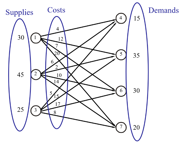
Using what we learned in Topic 6, we can write this out as a linear program using our canonical model
\[\begin{align*} Ax &= b, \tag{7.1}\label{eq:mato-7-1} \\ x &\leq u, \tag{7.2}\label{eq:mato-7-2} \\ x &\geq 0. \tag{7.3}\label{eq:mato-7-3} \end{align*}\]Writing out the constraints gives us
\[\sum_{j}x_{ij} = R_{i} \quad \text{for } i = 1,2,3, \tag{7.4}\label{eq:mato-7-4}\] \[\sum_{i}{x_{ij}} \leq D_{j} \quad \text{for } j = 4,5,6,7, \tag{7.5}\label{eq:mato-7-5}\] \[x_{ij} \geq 0 \quad \text{for } i = 1,2,3 \text{ and } j = 4,5,6,7. \tag{7.6}\label{eq:mato-7-6}\]If you want to teach the simplex method, a nice way is to use the network above and show the steps of simplex graphically, rather than the usual treatment using matrices. We are going to start by having all the flows exit through a super sink with zero-cost links moving from each destination node (nodes 4-7) with upper bounds equal to the demand at the node:
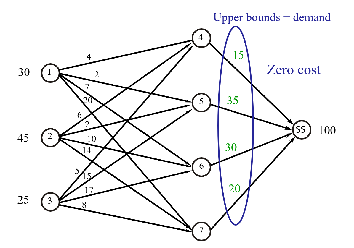
The supersink, while not necessary for the algorithm, will help to simplify the presentation.
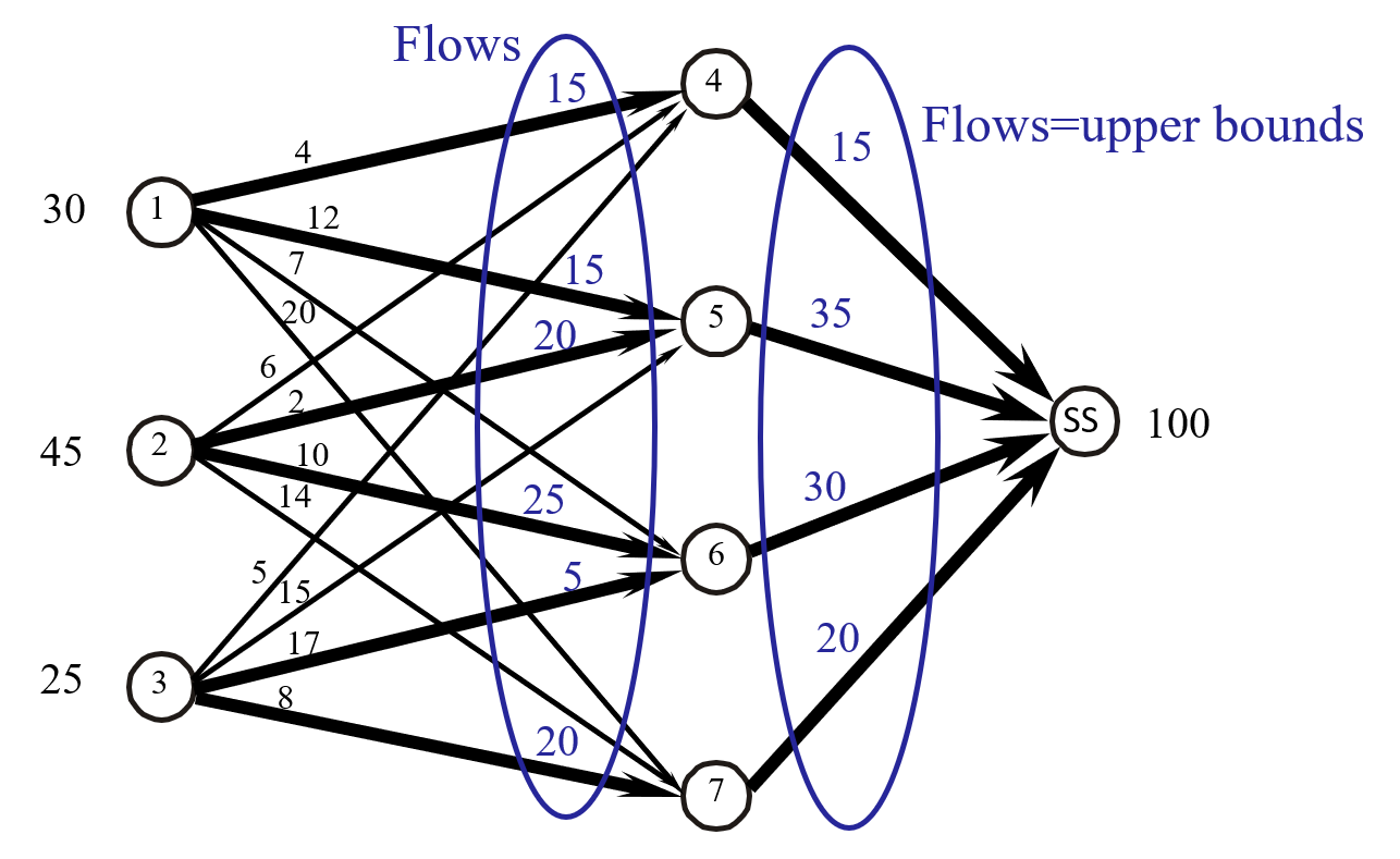
We first need an initial feasible solution, and this solution has to represent what is known as a basis. A basis (for a network problem) is a set of links with flows that satisfy all flow conservation constraints, along with all upper and lower bounds.
There are different ways to get an initial feasible solution. For this network problem, we can start by putting the required flow into each destination node (nodes 4-7) on the link into the supersink. Then, we start at node 4, find a link from a supply node (node 1), and put as much flow on this link as we can. Since the demand at node 4 is only 15, we cannot put more than 15. Also, since the supply at node 1 is 30, we have to take the smaller of 30 and 15 and put this amount (15) on the link (1-4).
Now we go to node 1 where we still have 15 units of unassigned flow. Node 5 needs 35 units of flow, but we only have 15 remaining, so we put 15. Now we go to node 5, where we still have an unsatisfied demand of 20, and look to the next supply node, node 2, which has 45 units of available flow. We take 20 of these to put on the link (2-5) which now gives us our required flow of 35 into node 5.
Next we move to node 2 where we still have 25 unassigned units of flow. We turn to node 6 that needs 30 units of flow, and push all 25 units of flow from 2 to 5. We still need 5 more units of flow at node 6, so we move down to node 3 and take 5 out of the available 25 units of flow.
Finally, we move the remaining 20 units of flow at node 3 to node 7.
We are not quite done. To be a basis (for a network), the set of links in the basis must satisfy two conditions:
- All links with flow strictly between the upper and lower bound must be in the basis.
- The set of links in the basis must form a tree.
So, we quickly see our links fail condition 2 – the set of links with flow do not form a tree. But we are not required to keep links with flow if the flow is at the upper or lower bound. Of the four links into the supersink, only one can be in the basis, so we are going to arbitrarily choose the first one, which gives us the basis:
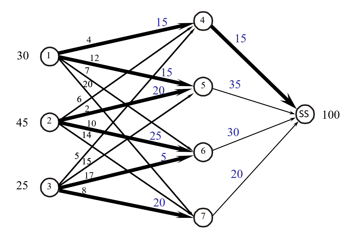
We are not claiming that this is optimal (it is not), but we now have a way of finding the optimal solution. The first step is to compute a “value” (known as a “dual variable”) which is the cost of moving a unit of flow from each node to the supersink. Remember that all the links directly attached to the supersink have 0 cost. So, the value at node 4 would be 0, since this is the cost of the path from 4 to SS.
To get from node 1 to SS, we have to move 1-4 (cost 4) and then 4-ss (cost 0) which is a cost of 4. A better way to get the dual at node 1 is to see that the path moves from 1 to 4 (at a cost of 4), and then just add the dual at 4 (which is 0).
To get from node 5 to SS, we first have to go backwards on the link (1-5), so this is a cost of minus 12. The dual at 1 is 4, so the dual at 5 is -12 + 4 = -8.
The dual at node 2 would be the cost of 2 to get 2-5, plus the dual at 5 = -8, so the dual at 2 = 2 + (-8) = -6. Continuing this logic for the remaining nodes gives us the duals:
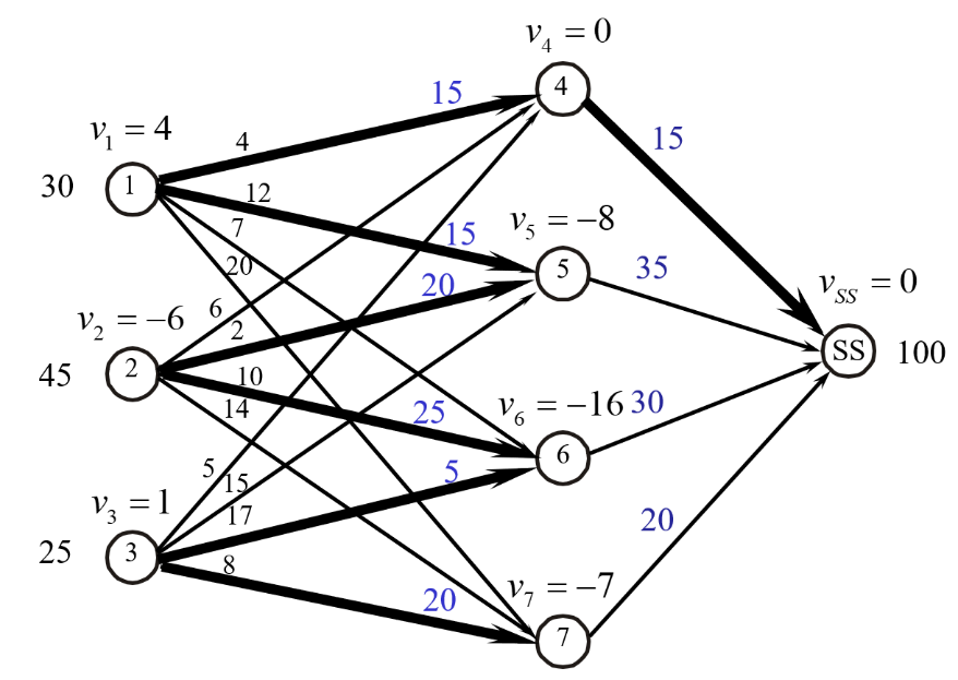
You can quickly check that each dual $v_{i}$ is the cost from that node to the supersink, following links that are in the basis.
Note at the same time there is always a single path from each node to the basis. This is a key property of the basis, which we are about to exploit.
Now let’s optimize. We are going to do this by looking at the nonbasic links without flow, and ask: What is the value of increasing flow on a nonbasic link?
Let’s take the link (1-6). To move one more unit of flow from 1 to 6, we are going to first add the flow from 1-6 (at a cost of 7), then we are going to move one unit of flow from 6 to the super sink, at a cost $v_{6} = -16$ (the dual variable for node 6), and then we are going to move one unit of flow from the super sink back to node 1. The cost of moving flow from SS to node 1 is negative the dual for node 1 (since this is the cost to go from 1 to SS). This means moving a unit of flow from 1 to 6, then 6 to SS, and finally SS back to 1, is
\[\bar{c}_{16} = c_{16} + v_{6} - v_{1}.\]The cost $\bar{c}_{16}$ is called the reduced cost since the cost is “reduced” by the changes needed to guarantee that we still satisfy all the constraints. This is a very simple calculation, which means we can do this calculation for every link that is not in the basis (note that the reduced cost for any link in the basis is equal to zero). For link 1-6, the reduced cost is
\[\bar{c}_{16} = c_{16} + v_{6} - v_{1} = 7 + (-16) - 4 = -13.\]The reduced cost captures the change in all the costs if we add one more unit of flow from 1 to 6, and then make all the other adjustments needed to ensure that we are still satisfying all the other constraints. Since the reduced cost is negative, this means that for each unit of flow, total costs will go down by 13, which means we get a better solution.
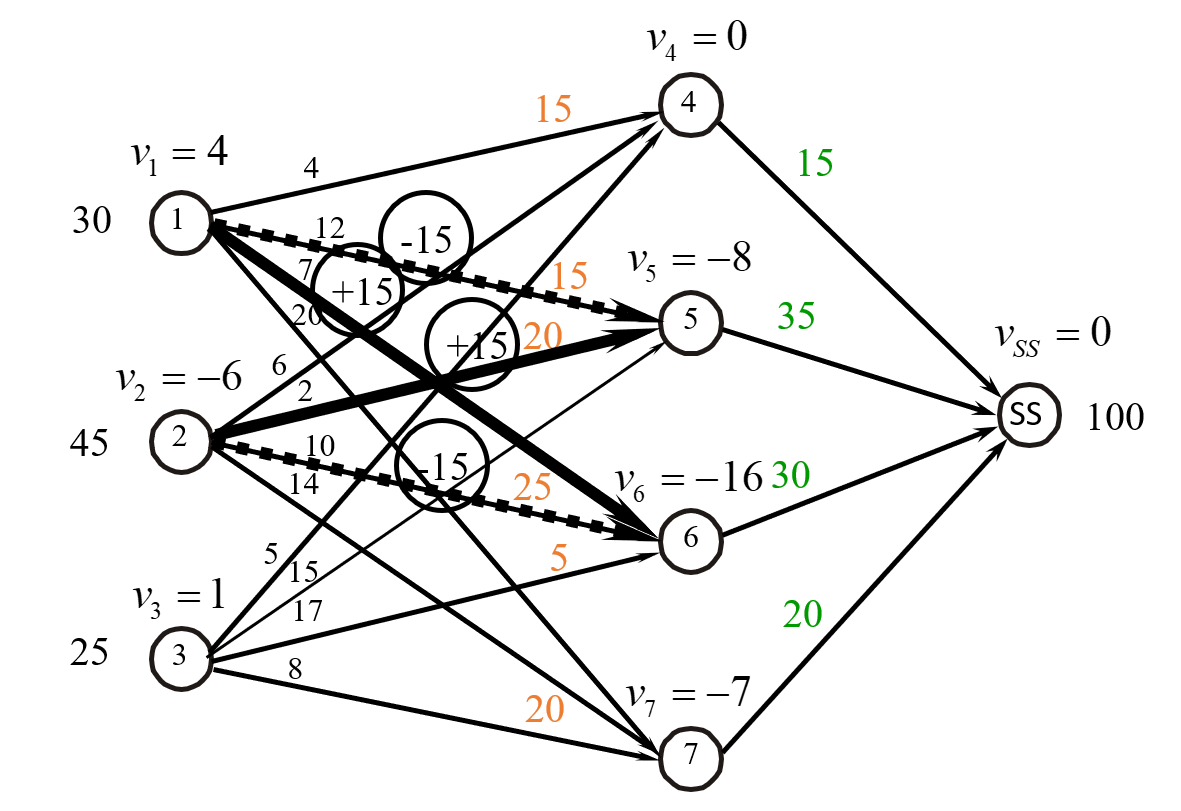
Now we just have to figure out how much flow we can move. We first note that adding one unit of flow from 6 to SS, and then moving one unit of flow from SS to 1, means there is no change on links 1-4 and 4-SS. The only links where flow actually changes are the links on the path along the links in the basis from 6 back to 1. This means flow increases on the links 1-6 and 2-5, while flow decreases on links 1-5 and 2-6. We want to move flow until the first link hits its lower bound (or upper bound if we had these, but we don’t). The link 1-5 has 15 units of flow, while link 2-6 has 25 units of flow, so link 1-5 will be the first link to hit zero. This means we can move 15 units of flow, at which point we would stop and drop link 1-5 from the basis (since it no longer has flow), while we now add link 1-6 to the basis.
We now have a new basis which means we have to update all our dual variables $v_{i}$. There are ways to do this very quickly, but these are technical issues that are not important for our discussion. Remember – we are not trying to teach students how to code the simplex algorithm – we are trying to teach important concepts in optimization.
With the new dual variables, we now have to recompute the reduced costs for all the nonbasic links (note that linear programming packages have tricks to do this very quickly). If we find another link with a negative reduced cost, then we have to repeat this exercise. We keep doing this until we no longer find any links with a negative reduced cost. At this point, we have found the optimal solution.
It is possible that when we route flow around the cycle, two links may hit zero at the same time. If this happens, we drop only one from the basis, and leave the other link with zero flow in the basis. This is known as a degenerate basis. A byproduct of a degenerate basis is that it is possible that we may find that the amount of flow we can move around the cycle (when we find a nonbasic link with negative reduced cost) is zero. Nothing wrong with this – it is actually fairly common.
This is a peek into the simplex method for network problems. The simplex algorithm works for linear programs that are not networks, and in this case we cannot draw these pretty pictures. But the basic idea is the same. Modern implementations of the simplex algorithm involve a vast array of engineering tricks to make the algorithm extremely fast. What is most important for students to understand is that we have exceptionally fast algorithms for solving linear programs, and free software is widely available.
Next, we are going to illustrate a dynamic inventory problem where we repeatedly solve linear programs over time.
7.2 The simplex algorithm II – with the matrix linear algebra
For a first course on optimization, I do not think it is necessary to show the matrix linear algebra behind the simplex algorithm, but there will be instructors who will want to include this material. This section includes all the slides from one of my lectures that presents the network simplex algorithm alongside the matrix calculations. You can download the PowerPoint slides that contain this material from https://tinyurl.com/PowellNetworkSimplex/.
The illustration below uses the network in section 7.1, but without the supersink. We choose node 1 arbitrarily to be the root node (and we explain why we need the concept of a “root node” for networks in the discussion below).
A generic linear programming model for a network problem is written as
\[\min_{x} \sum_{\text{supplies } i} \sum_{\text{demands } j} c_{ij}x_{ij}\]subject to the constraints:
\[\begin{align*} \sum_{j}{x_{ij}} &= S_{i} = \text{supply at node } i, \\ \sum_{i}x_{ij} &= D_{j} = \text{demand at node } j, \\ x_{ij} &\geq 0. \end{align*}\]We can write these constraints in matrix form as $Ax = b$, $x \geq 0$.
Now assume we are going to solve the numerical example below.
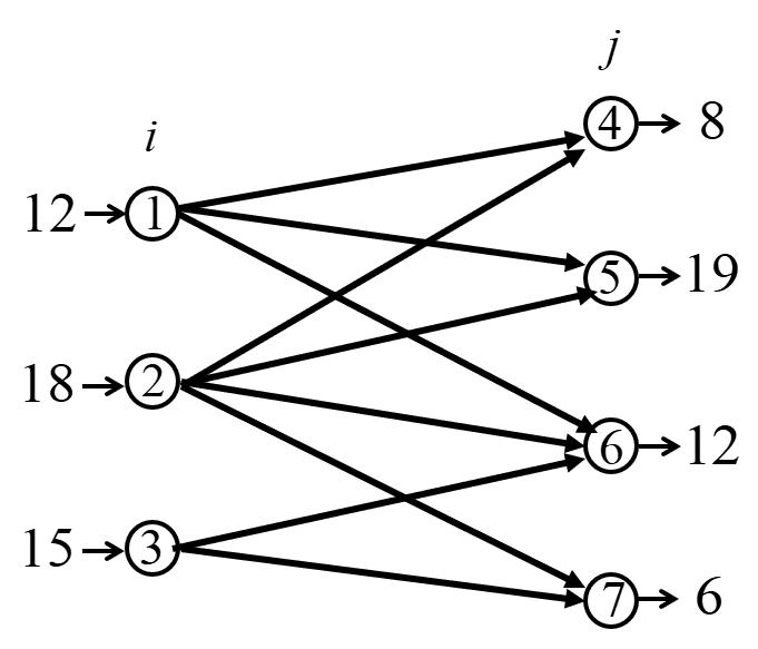
Our constraints would look like
\[x_{14} + x_{15} + x_{16} = 12\] \[x_{24} + x_{25} + x_{26} + x_{27} = 18\] \[x_{36} + x_{37} = 15\] \[-x_{14} - x_{24} = -8\] \[-x_{15} - x_{25} = -19\] \[-x_{16} - x_{26} - x_{36} = -12\] \[-x_{27} - x_{37} = -6\] \[x_{14},x_{15},x_{16},x_{24},x_{25},x_{26},x_{27},x_{36},x_{37} \geq 0\]We would write our constraint matrix $A$ with a row for each constraint, and a column for each variable $x_{ij}$, giving us the matrix:
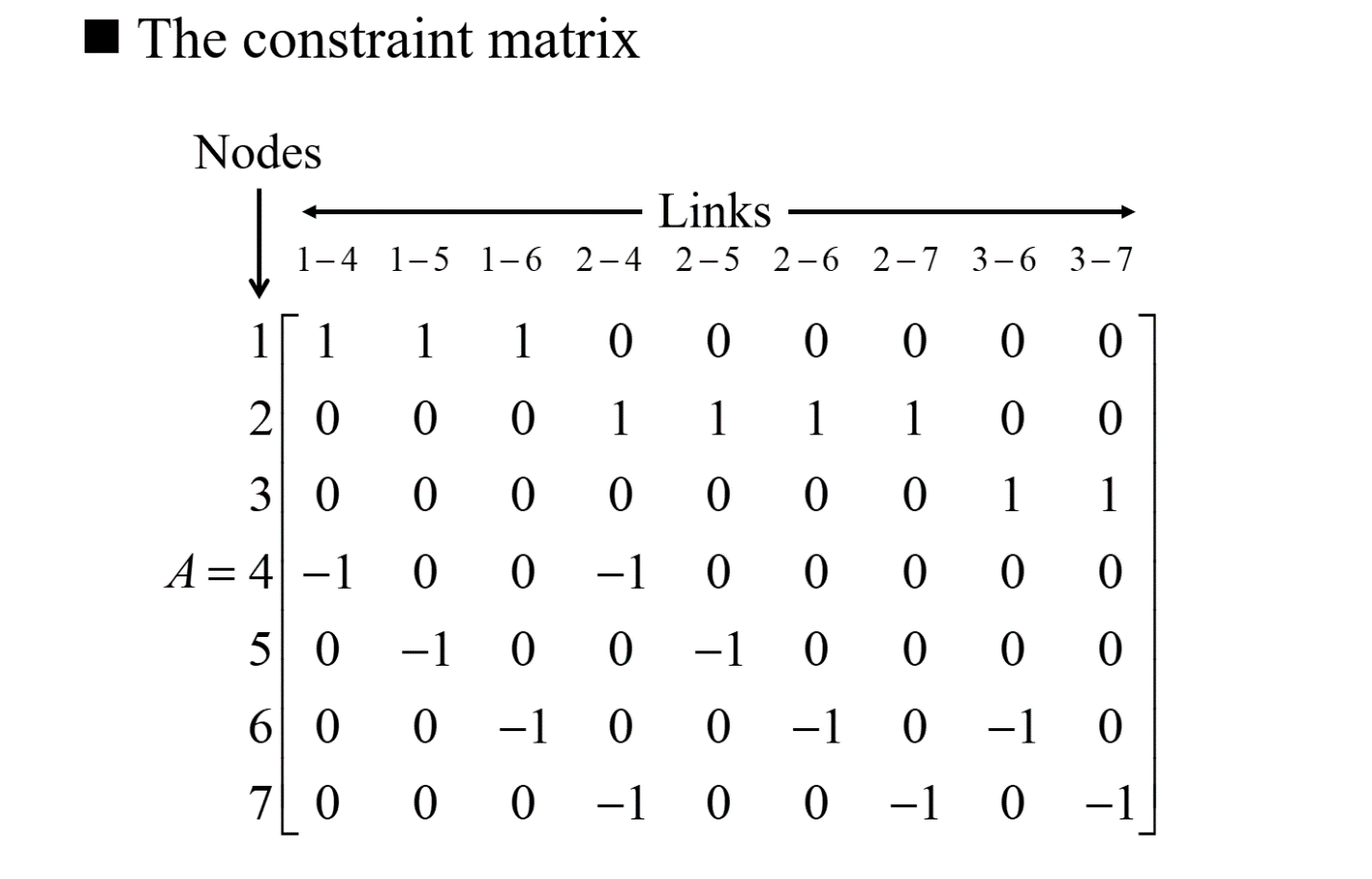
Some notes:
- If we add the rows of the matrix $A$, they sum to zero. This means that one of the rows is redundant. If we drop one of the rows, all the constraints will still be satisfied. In other words, if we have a network with $n$ nodes, we need $n-1$ constraints.

The simplest way to illustrate this property of networks is to consider a network with two nodes and one link, as shown above. If we enforce flow conservation at node 1, this means we will be sending 6 units of flow from 1 to 2, which automatically satisfies the flow conservation constraint at node 2.
- So, for larger networks, we can pick any node and drop its constraint. This node is called the root node. If $r$ is the root node, then the dual variable $v_{r} = 0$ (remember – this is the cost of moving a unit of flow from that node to the root node).
- For our network above, we can arbitrarily pick node 1 as the root node. This gives us the following constraint matrix:
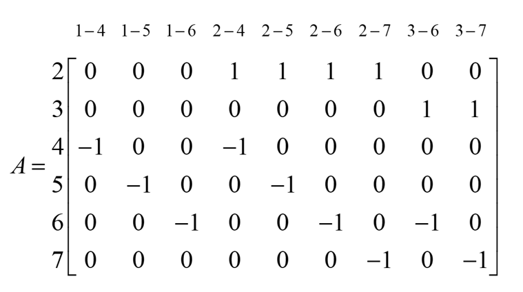
The simplex algorithm for linear programming requires that we start with a basis which is a set of variables $x_{ij}$ which we are going to adjust to guarantee that the constraints are satisfied any time we change a variable that is not in the basis. Our only requirement for a nonbasic variable is that it must be at its lower or upper bound. In our numerical example (without the supersink), we do not have any variables with upper bounds, so all nonbasic variables must equal 0.
These concepts are best explained by example.
We have to start by creating our basis. We need to find a set of flows that satisfies the constraints. We do not care about the quality of the solution – our simplex algorithm can start with any feasible solution that satisfies the rules for our basic and nonbasic variables.
Professional linear programming packages have sophisticated logic for creating starting solutions. For our simple problem, we are going to use a simple strategy called the “northwest corner rule” where we literally start in the northwest corner of our graph (that is, node 1), and start assigning flow to the northeast corner (which would be node 4). We assign as much as we can (that is, the smaller of either the supply at node 1 or the demand at node 4). We then move to either the next supply node (if we allocated all the supply from node 1) or the next demand node (if we satisfied all the demand at node 4), and keep repeating the process using the remaining nodes with unused supply or unsatisfied demand. This process produces the network below, along with the basic vector $x^{B}$ (the vector of links $x_{ij}$ for links in the basis) and the nonbasic vector $x^{N}$ (the links not in the basis):
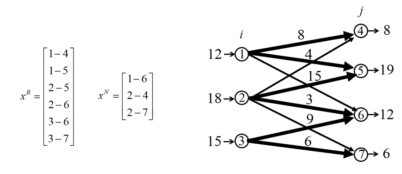
We can now partition our $A$-matrix into a square matrix $A^{B}$ of the basic variables (it will always be square) and the remaining matrix $A^{N}$ comprised of the non-basic columns:
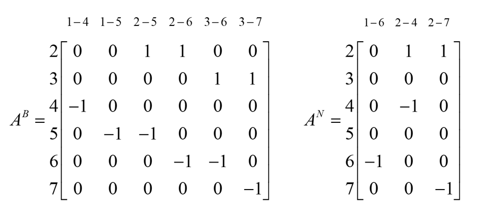
We can now restate our constraints using the vectors of basic and nonbasic variables, and the corresponding columns of the $A$ matrix. The constraints $Ax = b$ become
\[\begin{bmatrix} A^{B} & A^{N} \end{bmatrix}\begin{bmatrix} x^{B} \\ x^{N} \end{bmatrix} = b,\]which is the same as
\[A^{B}x^{B} + A^{N}x^{N} = b.\]We can now solve for the basic variables $x^{B}$ in terms of the nonbasic variables $x^{N}$:
\[x^{B} = \left[ A^{B} \right]^{-1}\left[ b - A^{N}x^{N} \right].\]For our network problem, we have no upper bounds so $x^{N} = 0$, but this will not always be the case. Note that we can guarantee that the matrix $A^{B}$ is, in fact, invertible by how we have constructed the basis.
For general linear programming problems we need some reasonably sophisticated linear algebra to handle the matrix inversion $\left[ A^{B} \right]^{-1}$. Remember that linear programming models have been solved with millions of variables. In fact, network problems (which have a lot of structure) can be solved even with tens of millions of variables. We would not even be able to store a matrix $A^{B}$ with millions of rows and columns. This is where specialists use a lot of tricks.
In fact, we are going to show you how you can invert the basis matrix $A^{B}$ for our network problem by inspection!
Recall that each row of the basis matrix $A^{B}$ corresponds to a node, while each column corresponds to a link (that is, a decision variable $x_{ij}$). This is why we often call $A^{B}$ a “node-arc incidence matrix.” It turns out that each row of the inverse $\left[ A^{B} \right]^{-1}$ corresponds to a link, while each column corresponds to a path from a node to the root node. The element of the matrix $\left[ A^{B} \right]^{-1}$ indicates if the link for that row is in the path from the node for that column. We use 0 if the link is not in the path, and then +1 or -1 to indicate if the link is in the path, and whether you have to traverse the link in the forward direction or backwards. The choice of whether it is +1 or -1 depends on what sign convention you have used in your flow conservation constraints (that is, did you write flow out minus flow in, or the reverse). Below is the inverse that we get for our problem.
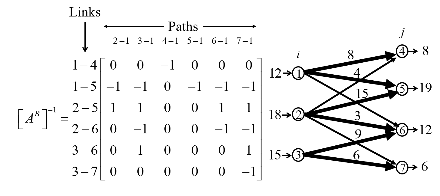
To verify that $\left[ A^{B} \right]^{-1}$ is in fact the inverse of $A^{B}$, we can perform the multiplication $A^{B}\left[ A^{B} \right]^{-1}$ to verify that we get the identity matrix. This is done below:
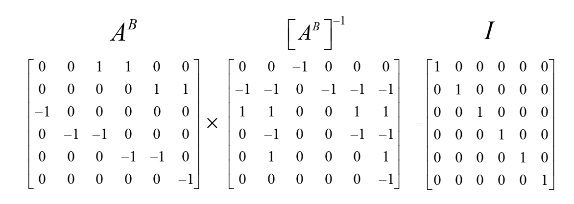
Note that if we perform this multiplication and find we get $-I$ then you just have to switch your sign convention. Obviously you only have to check this for one element.
We can rewrite our objective function using
\[\min_{x} c^{T}x = \left( c^{B} \right)^{T}x^{B} + \left( c^{N} \right)^{T}x^{N}\] \[= \left( c^{B} \right)^{T}\left( \left[ A^{B} \right]^{-1}(b - A^{N}x^{N}) \right) + \left( c^{N} \right)^{T}x^{N}\] \[= \left( c^{B} \right)^{T}\left[ A^{B} \right]^{-1}b - \left( c^{B} \right)^{T}\left[ A^{B} \right]^{-1}A^{N}x^{N} + \left( c^{N} \right)^{T}x^{N}\] \[= \left( c^{B} \right)^{T}\left[ A^{B} \right]^{-1}b + \bar{c}^{N}x^{N},\]where $\bar{c}^{N}$ is the vector of “reduced costs” for the nonbasic links given by
\[\bar{c}^{N} = \left( c^{N} \right)^{T} - \left( c^{B} \right)^{T}\left[ A^{B} \right]^{-1}A^{N}.\]Reduced costs tell us if we should increase the flow on a nonbasic link, while adjusting flows on all the basic links so that the flow conservation (plus upper and lower bound) constraints are satisfied. For our numerical example above, the reduced costs are calculated as follows:
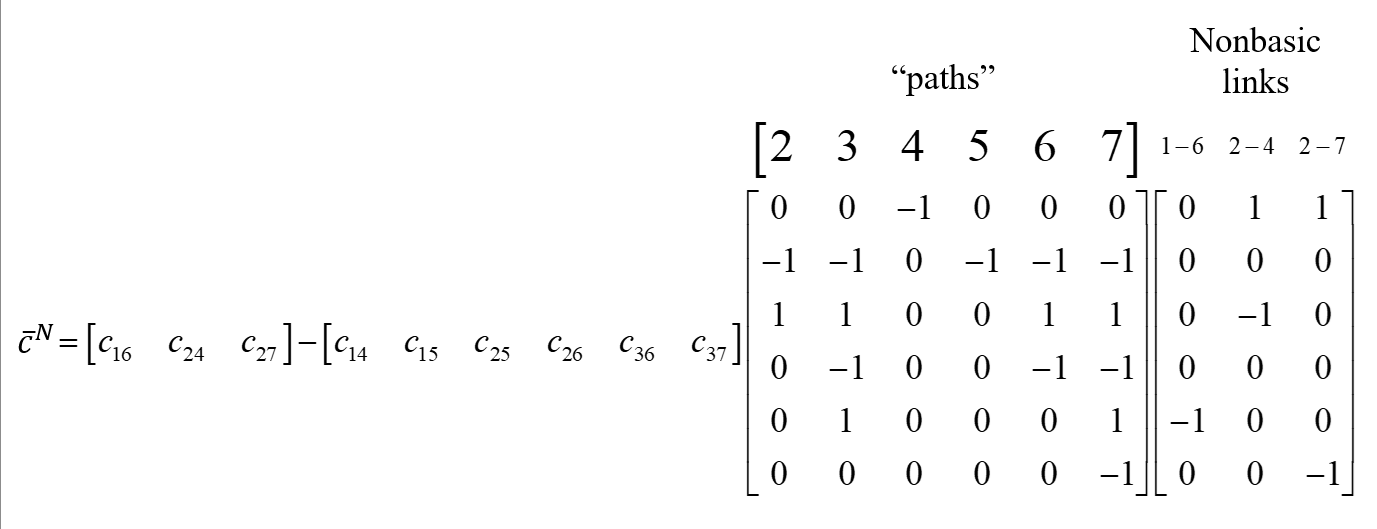
Continuing the calculations:
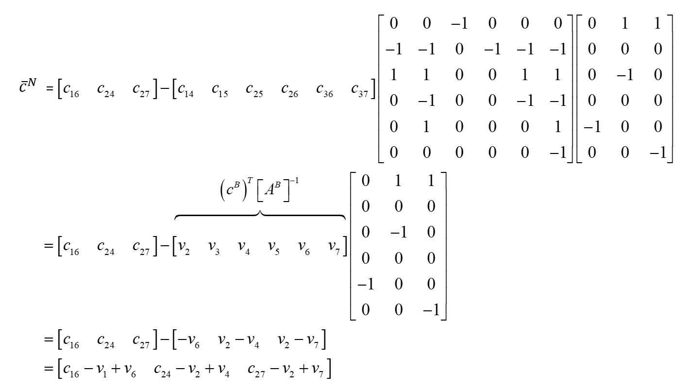
We see that $\left( c^{B} \right)^{T}\left[ A^{B} \right]^{-1}$ is the inner product of the link costs (for basic links) times the link-path incidence matrix $\left[ A^{B} \right]^{-1}$. This means that $\left( c^{B} \right)^{T}\left[ A^{B} \right]^{-1}$ is the vector of dual variables, which as we have seen are the path costs along the basis from each node to the root node. All of this reduces to the simple relationship (for networks) between costs and reduced costs for nonbasic links
\[\bar{c}^{N} = \begin{bmatrix} c_{16} - v_{1} + v_{6} & c_{24} - v_{2} + v_{4} & c_{27} - v_{2} + v_{7} \end{bmatrix}.\]We can compute the path costs (dual variables) $v_{i}$ just by following the path along the basis from each node to the supersink (node 1). Remember we have to subtract the cost for any link that we traverse in the reverse direction of the link.
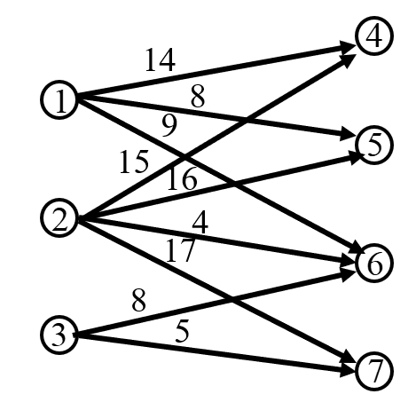
This gives us
\[\begin{align*} v_{1} &= 0, \\ v_{2} &= 16 - 8 = 8, \\ v_{3} &= 8 - 4 + 16 - 8 = 12, \\ v_{4} &= -14, \\ v_{5} &= -8, \\ v_{6} &= -4 + 16 - 8 = 4, \\ v_{7} &= -5 + 8 - 4 + 16 - 8 = 7. \end{align*}\]The reduced costs on the nonbasic links are then
\[\begin{align*} \bar{c}^{N} &= \begin{bmatrix} \bar{c}_{16} & \bar{c}_{24} & \bar{c}_{27} \end{bmatrix} \\ &= \begin{bmatrix} c_{16} - v_{1} + v_{6} & c_{24} - v_{2} + v_{4} & c_{27} - v_{2} + v_{7} \end{bmatrix} \\ &= \begin{bmatrix} 9 - 0 + 4 & 15 - 8 + (-14) & 17 - 8 + 7 \end{bmatrix} \\ &= \begin{bmatrix} 13 & -7 & 16 \end{bmatrix}. \end{align*}\]The reduced cost tells us how much total costs will change if we increase the flow on each nonbasic link. If the reduced cost is negative, we get a better solution by increasing flow on that link. We now search for nonbasic links with a negative reduced cost, since this means increasing the flow on that link, and then adjusting the flows on the basic links so we maintain flow conservation, will reduce total costs.
There are different strategies for choosing the nonbasic link, since networks can be quite large (from many thousands of links to millions of links). It makes sense to choose the nonbasic link with the most negative reduced cost, but this would mean calculating all the reduced costs and finding the smallest. Computer scientists have refined these strategies to balance the time required to find the best nonbasic link that produces the fastest convergence.
From our list of reduced costs above, we see that the only nonbasic link with a negative reduced cost is link (2,4). We want to increase flow from 2 to 4. Then, to maintain flow conservation, for each unit of flow we push from 2 to 4, we want to push a unit from 4 to the root node (node 1), and then from the root node to node 2, always limiting ourselves to links in the basis. We note that there is always exactly one path between any node and the root node.
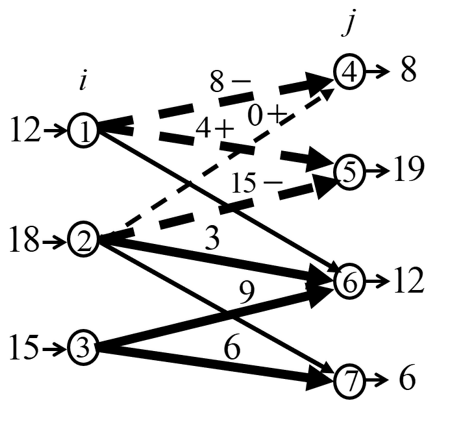
As we see the graph, the path from 4 to the root node means reducing a unit of flow on the link from 1 to 4. Then, we have to push a unit of flow from node 1 to node 2, which means increasing flow on link (1,5) and then decreasing flow on link (2,5).
The next step is that we have to figure out how much flow to move. The answer to this is simple: we move as much as possible. We look at each link that is losing flow, and then calculate how much flow is on these links, and take the link with the smallest flow. If links have upper bounds, then we also look at each link that is gaining flow, and take the link that can increase flow by the smallest amount before hitting the upper bound. Finally, we choose the link that can lose (or gain) the smallest amount of flow, and that link determines how much flow we can lose. The constraining link is also the link that we drop from the basis.
After we complete the process of adding the new nonbasic link and dropping the constraining link, we have to recompute the dual variables $v_{i}$. Again, we note that commercial software uses a variety of programming tricks to accelerate this process.
Some notes:
- It is possible that there may be a tie – two links losing flow have the same amount of flow, or the link that can lose the least flow matches the link that can gain the least flow. In case of ties, we just pick one link arbitrarily to drop from the basis. After adding the new nonbasic link, we regain a valid basis (that is, all the links in the basis always form a tree).
- It is also possible that the amount of flow that we can move is zero. This can (and will) happen, and is known as a “degenerate pivot.” Even when the amount of flow we can move is zero, we still go through the same process of adding the new nonbasic link to the network, and dropping one of the constraining links (if there is more than one).
We note that all of our calculations seem to depend on our choice of root node. It turns out that changing the root node has the effect of changing all of the dual variables by a constant, which means that the reduced costs, which all involve differences between dual variables, are not affected. Below are two networks with different root nodes to illustrate this property.
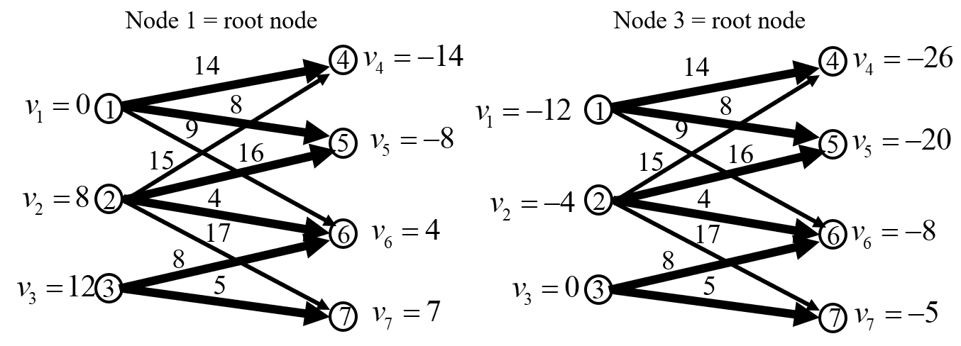
This nice property also hints at a limitation in the interpretation of a dual variable. It is common to think of a dual variable $v_{i}$ as being the marginal value of the resources entering or leaving the network at node $i$. Since the sum of the supplies and demands for our network problem must sum to zero, it does not make sense to perturb the flow entering or leaving the network at node $i$, since we also have to specify the change in the flow at some other node so that the supplies and demands remain balanced. We have actually addressed this problem by dropping one of the constraints (the root node). This means that if we perturb the supply or demand at some node $i$, we are implicitly balancing this change by adding or subtracting the same amount of flow at our root node so that the sum of supplies and demands remain balanced.
7.3 As a policy for a dynamic problem
Let’s start with the same network problem we used above, but now assume that we are using this to match available inventories of products in distribution centers to the demands of retailers looking to restock their inventories. We might reasonably solve this problem daily (or weekly), but in this case we are now solving a sequential decision problem, where our “policy” requires solving the linear programming problem.
Recognizing that we are solving this problem each time period, our optimization problem at time $t$ would be written
\[\min_{x_{t}}{\sum_{i,j}{c_{tij}x_{tij}}}\]subject to
\[\sum_{j}x_{tij} = R_{ti} \quad \text{for } i = 1,2,3, \tag{7.7}\label{eq:mato-7-7}\] \[\sum_{i}{x_{tij}} \leq D_{tj} \quad \text{for } j = 4,5,6,7, \tag{7.8}\label{eq:mato-7-8}\] \[x_{tij} \geq 0 \quad \text{for } i = 1,2,3 \text{ and } j = 4,5,6,7, \tag{7.9}\label{eq:mato-7-9}\]where the supplies at time $t$ are given by $R_{ti}$ and the demands are given by $D_{tj}$. We have also allowed our costs $c_{t}$ to be time-dependent. We quickly see that we can minimize costs by not satisfying any demand, so a better model might be to maximize profits. Let $p_{tj}$ be the price we receive for satisfying a unit of demand at node $j$. Our objective function would then be
\[\max_{x_{t}}\left( \sum_{j}{p_{tj}\min\left\{ D_{tj},\sum_{i}x_{tij} \right\}} - \sum_{i,j}{c_{tij}x_{tij}} \right) \tag{7.10}\label{eq:mato-7-10}\]A more realistic model needs to be modified to reflect the possibility that total supply may be greater than total demand, or less than total demand. We have already written the demand constraint $\eqref{eq:mato-7-8}$ as an inequality. However, we need to add the option that allows us to hold excess inventory until time $t+1$. In fact, we may even want to hold inventory while not satisfying demand. Remember that in our model we are allowing costs and prices to vary over time. There may be a time period where costs rise and/or prices drop, at which point we prefer to hold our inventory for a future time period when prices and costs may be more favorable.
We may face uncertainty in our available inventories (these might include inventories arriving soon, but perhaps they are delayed), or the demands (which may be higher or lower than expected). We might, then, replace constraints $\eqref{eq:mato-7-7}$-$\eqref{eq:mato-7-9}$ with
\[\sum_{j}x_{tij} = \theta^{R}R_{ti} \quad \text{for } i = 1,2,3, \tag{7.11}\label{eq:mato-7-11}\] \[\sum_{i}{x_{tij}} \leq \theta^{D}D_{tj} \quad \text{for } j = 4,5,6,7, \tag{7.12}\label{eq:mato-7-12}\] \[x_{tij} \geq 0 \quad \text{for } i = 1,2,3 \text{ and } j = 4,5,6,7. \tag{7.13}\label{eq:mato-7-13}\]The objective function $\eqref{eq:mato-7-10}$ with constraints $\eqref{eq:mato-7-11}$-$\eqref{eq:mato-7-13}$ looks like another optimization problem, but there is an important difference. This is just a problem at time $t$, where we want to maximize profits over time, not just at a point in time. If we choose to maximize $\eqref{eq:mato-7-10}$ to get our decisions of what to do at time $t$, then we would say that this problem is now a policy which should be written
\[X^{\pi}\left( S_{t} \middle| \theta \right) = \underset{x_{t}}{\arg\max}\left( \sum_{j}{p_{tj}\min\left\{ D_{tj},\sum_{i}x_{tij} \right\}} - \sum_{i,j}{c_{tij}x_{tij}} \right) \tag{7.14}\label{eq:mato-7-14}\]which has to be solved subject to the constraints $\eqref{eq:mato-7-11}$-$\eqref{eq:mato-7-12}$. Using $\eqref{eq:mato-7-14}$ as a policy completely ignores the impact of decisions now on the future. For example, imagine that at time $t$ the prices $p_{t}$ are unusually low. Thus, we can use our simplex algorithm to find the optimal solution of our linear program, but solving $\eqref{eq:mato-7-14}$ is not an optimal policy!
We might create a more sophisticated policy by optimizing into the future, just as we did in our dynamic shortest path problem where we would plan a path to the destination, which would then be updated as new information came in. Such a direct lookahead (DLA) policy could be written
subject to, for $t’ = t,\ t+1,\ \ldots,\ t+H$:
\[\sum_{j}\tilde{x}_{tt'ij} = \theta^{R}\tilde{R}_{tt'i} \quad \text{for } i = 1,2,3, \tag{7.16}\label{eq:mato-7-16}\] \[\sum_{i}{\tilde{x}_{tt'ij}} \leq \theta^{D}\tilde{D}_{tt'j} \quad \text{for } j = 4,5,6,7, \tag{7.17}\label{eq:mato-7-17}\] \[\tilde{x}_{tt'ij} \geq 0 \quad \text{for } i = 1,2,3 \text{ and } j = 4,5,6,7. \tag{7.18}\label{eq:mato-7-18}\]Note that we have put tildes on all the variables used to plan into the future. Also, each of the tilde-variables has two time indices: time $t$, since we are solving the problem at time $t$, and time $t’$, which is the time we are planning into the future. Other variables such as prices or demands are forecasts of future prices or demands made at time $t$.
Note that we do not care about the entire optimal solution over the horizon $t,\ \ldots,\ t+H$. We are only going to implement the first time period, which means we would set
\[x_{t} = \tilde{x}_{tt}.\]Note that our DLA policy in $\eqref{eq:mato-7-15}$-$\eqref{eq:mato-7-18}$ is still not an optimal policy, but it might be quite good. One challenge is that we have to tune the parameters $\theta = (\theta^{R},\theta^{D})$.
We need to first write out how we would simulate our policy $X_{t}^{\pi}\left( S_{t} \middle| \theta \right)$. This requires identifying how random events (e.g. random demands, travel times, …) affect how the solution $x_{t}$ behaves in practice. This is a key step that is almost always overlooked when modeling and solving linear programs. What you have to do is to imagine that you are simulating the process. These equations represent the transition function in our sequential decision model which we represent compactly as
\[S_{t + 1} = S^{M}\left( S_{t},x_{t},W_{t + 1} \right).\]Assume as we have done before that we can generate a series of sample paths where the $n^{\text{th}}$ sample path is
\[\omega^{n} = (W_{1}^{n},W_{2}^{n},\ldots,W_{T}^{n}).\]Let $S_{t}^{n}$ be the state at time $t$ while we are following sample path $\omega^{n}$. Specifying $\omega^{n}$ refers to a specific sample of anything random (demands, prices, travel times, …). The value of the policy for sample path $\omega^{n}$ might be written
\[F^{n}(\theta) = \sum_{t = 0}^{T}{C(S_{t}(\omega^{n}),X_{t}^{\pi}(S_{t}(\omega^{n})|\theta))},\]where $X_{t}^{\pi}(S_{t}(\omega^{n})|\theta)$ is the policy computed from $\eqref{eq:mato-7-15}$-$\eqref{eq:mato-7-18}$. If we generate $n = 1,\ \ldots,\ N$ sample paths, we can evaluate the policy by taking an average
\[\bar{F}^{\pi}(\theta) = \frac{1}{N}\sum_{n = 1}^{N}{\sum_{t = 0}^{T}{C(S_{t}(\omega^{n}),X_{t}^{\pi}(S_{t}(\omega^{n})|\theta))}}.\]There are, of course, different ways to parameterize the policy. This means that when we optimize over policies, it requires designing different parameterizations, and then tuning each one. Let $f \in F$ be a family of parameterizations (we have to make these up by hand), and let $\theta \in \Theta^{f}$ be the parameters for parameterization $f$. Our policy $\pi = (f,\theta)$ consists of the parameterization and its tunable parameters.
We can now write out our optimization problem as
\[\min_{\pi = (f,\theta)}{\bar{F}^{\pi}(\theta)}.\]This discussion has illustrated that we are going to need to identify and compare different types of policies (such as $\eqref{eq:mato-7-15}$-$\eqref{eq:mato-7-18}$) as well as tuning any parameters that we have inserted. Coming up with different types of policies parallels choosing between the linear and nonlinear models we illustrated in Topic 1 on machine learning. Tuning the parameters for the policies parallels fitting our parametric models in machine learning.
While this process may seem ad hoc, it is no more ad hoc than searching among different statistical models in machine learning. Furthermore, this is precisely how the vast majority of sequential decision problems are solved in practice.
Topic 8: Dynamic inventory problems – Energy storage
Readings: SDAM Chapter 9 – this is also where we introduce linear programming
Here we address a more complex energy storage problem: we have to decide how much to draw from a windfarm (with variable supply), the grid (with variable prices), to meet a predictable load (demand) for a building, using an energy storage device to absorb variations.
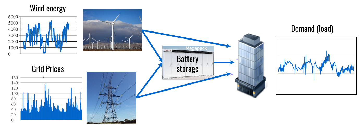
We have rolling forecasts of wind which change quite a bit from hour to hour:
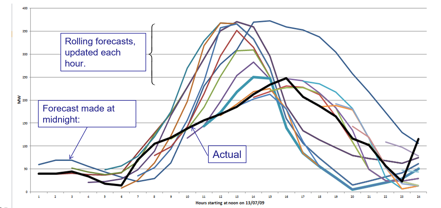
We are going to solve this much as we solve our dynamic shortest path problem, where we look into the future and pretend the various forecasts (such as wind) are perfectly accurate. This “lookahead model” is another example of a linear program. Even though the decision at each point in time is a scalar, we have to optimize the decisions over the entire horizon, which means we have to optimize over the entire vector of decisions.
Now, to handle uncertainty, we insert a coefficient $\theta_{t’ - t}$ for our forecast of wind made at time $t$, of what the energy from the wind farm will be at time $t’$. Note that $\theta_{t’ - t}$ is not a function of $t$, it is just a function of the difference $t’ - t$. So if we look 24 hours into the future, we would have 24 coefficients. A simpler strategy to get us started would be to assume that there is just one coefficient for all forecasts. The modified lookahead linear program looks like:
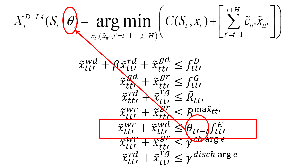
This closely parallels the idea of solving a shortest path with modified costs. We solved that problem using our shortest path algorithm. This time, we need the full power of a linear program that we introduced in Topic 7.
Our next challenge is to tune the parameter vector $\theta$ which could be a scalar (if we use one parameter for all the forecasts) or, in our case, a 24-dimensional vector (one for each hour into the future). We first need to write out how we are going to evaluate our policy. If $X_{t}^{D-LA}\left( S_{t} \middle| \theta \right)$ is our policy above, assume that it returns a decision vector $x_{t}$ that determines what to do right now.
Let $C(S_{t},x_{t})$ be our performance metric (e.g. total costs) that occur just at time $t$. Now let $W_{1},\ W_{2},\ldots,\ W_{t},\ldots,\ W_{T}$ be a sample realization of all the new information arriving, where $W_{t}$ is the information that arrives between $t-1$ and $t$. This would include energy from the wind farm, the grid price, along with the latest set of rolling forecasts of demands, grid prices and the energy from wind. If we have access to real data, we could use that. Otherwise, we would likely use Monte Carlo simulation which we described in Topic 2.
We need to write a simulator that we represent using our transition function
\[S_{t + 1} = S^{M}(S_{t},\ x_{t},W_{t + 1}),\]where $S_{t}$ captures everything we know at time $t$, our decision comes from our policy $x_{t} = X_{t}^{D-LA}\left( S_{t} \middle| \theta \right)$, and the new information $W_{t + 1}$ comes from our historical data or simulation. The transition function describes how our state variable changes over time (for example, this is where we update how much energy is in our storage device).
Running the simulation on the data $W_{t}$, with decisions from the policy $X_{t}^{D-LA}\left( S_{t} \middle| \theta \right)$, allows us to estimate the performance of the policy:
\[F^{D-LA}(\theta) = \sum_{t = 0}^{T}{C(S_{t},x_{t} = X_{t}^{D-LA}\left( S_{t} \middle| \theta \right))}.\]Next we have to turn to algorithms to search for the best value of $\theta$. If we assume there is only a single parameter $\theta$ for all time periods in the future, this would just be a one-dimensional search. If it is a vector, we could use a gradient-based search such as what we illustrated in Topic 1 for nonlinear models. (See section 5.4 in RLSO for a more thorough discussion of how to compute gradients numerically.)
We can set up our simulation so that the rolling forecast is perfectly accurate. In this case, we would expect the best value of $\theta$ to be 1.0. The figure below confirms this.
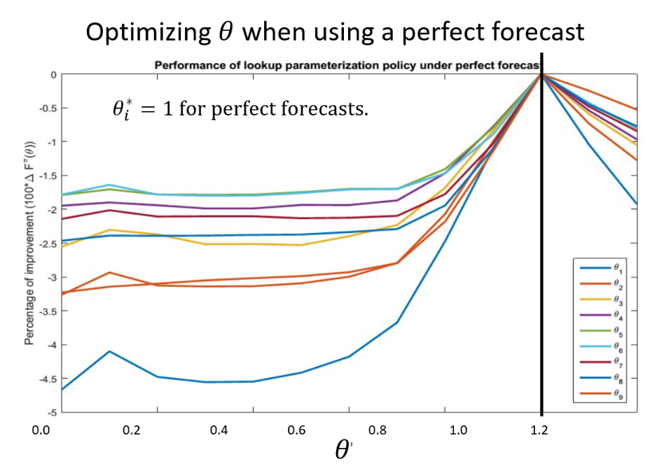
Now run the experiment where the rolling forecast (say of wind) is not accurate, as would occur in practice. In this case, we get the graph below, where the best values of $\theta$ are quite different from 1.0.
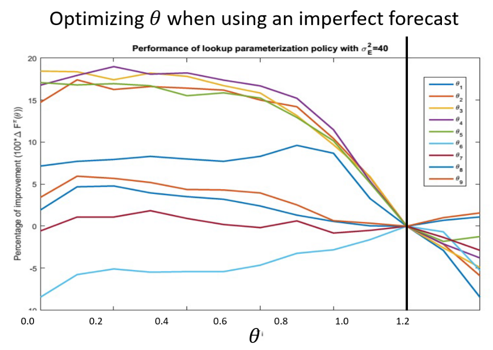
The figure below shows that we can achieve approximately a 30 percent improvement using optimized $\theta$.
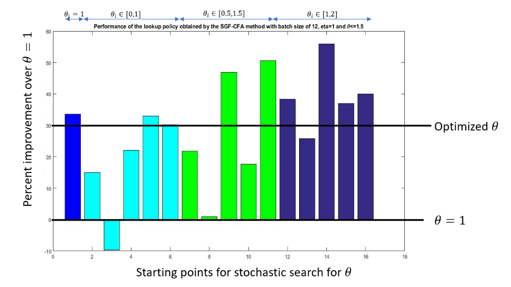
This application illustrates the very powerful idea of parameterizing an optimization problem. I suspect that there is a wide array of optimization problems that are actually policies for fully sequential problems. The idea of parameterizing an optimization problem is widely used in industry, but in an ad hoc way.
Topic 9: Integer programming
We now introduce integer programming, using the classic problem of a facility location problem. Some schools teach entire courses on integer programming, so this lecture is more of a placeholder. An instructor can cover this material very briefly (e.g. at the level of these notes), or delve into the richer modeling challenges. We note that as of this writing, the best integer programming solvers (such as Gurobi or Cplex) are quite powerful for a wide range of problems.
As we did with linear programming, we are going to start with a basic integer programming problem which can be solved using commercial packages. It is for this reason that, as with linear programming, the traditional emphasis on algorithms is simply not appropriate for an introductory course.
We are going to introduce integer programming using a classical (and widely used) application of optimizing a set of locations to build or lease warehouses. This is a problem that can be solved to near optimality by high quality commercial packages. Unlike linear programs, integer programs come in different flavors, some of which are easier to solve while others still require specialized algorithms. In section 9.2 we provide a summary of some of the major classes of integer programming problems.
As we did with linear programming, we start with static models to illustrate integer programming. We follow in Topic 10 by extending the facility location problem to a dynamic setting.
9.1 Static facility location
A problem faced by many companies is locating facilities – these might be manufacturing points, distribution centers, warehouses, and even retail locations (if the company is a retailer).
Imagine that we are trying to design the network in the graphic below. We might assume we have a known manufacturing location in Mexico, but we have to optimize the location of distribution centers (black squares) and local warehouses (the smaller circles). To model this problem, let:
| $I^{facility}$ | Set of candidate locations for distribution centers and warehouses (to be chosen). |
| $I^{prod}$ | Set of production facilities (fixed in advance). |
| $I^{retail}$ | Set of retailers where product is sold (fixed in advance). |
| $x_{ij}^{trans}$ | Flow of goods (in pounds per quarter) from $i$ to $j$; $x^{trans} = \left( x_{ij}^{trans} \right)_{i,j}$. |
| $x_{i}^{facility}$ | $1$ if we build facility $i$, $0$ otherwise, for $i \in I^{facility}$; $x^{facility} = \left( x_{i}^{facility} \right)_{i \in I^{facility}}$. |
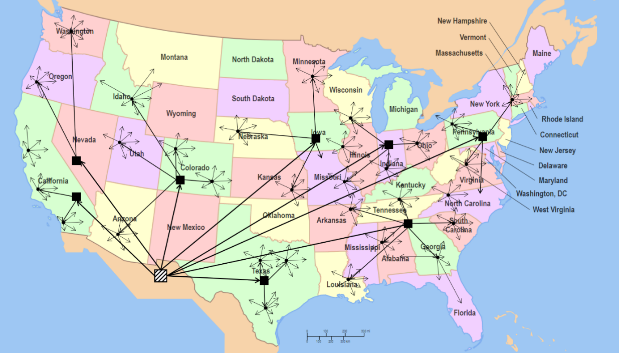
We can combine these into a single vector: $x = (x^{trans},x^{facility})$.
Next define the costs: $c_{i}^{facility}$ is the cost per quarter to lease/operate facility $i$, and $c_{ij}^{trans}$ is the transportation cost per pound for moving freight from $i$ to $j$.
We have to move the freight from places where we have supplies, which includes initial inventories as well as the ability to produce the product (presumably only at the manufacturing facility). For this we let $q_{i}^{prod}$ be the production capacity of manufacturing facility $i \in I^{manuf}$, where we assume there is sufficient production capacity to meet the total market demand. We then have to satisfy demands, given by $D_{i}$, the demand for goods (in pounds) at retailer $i$ over the quarter.
Our optimization problem to find the location of facilities can then be stated as
\[\min_{x = (x^{trans},x^{facility})}{\sum_{i \in I^{facility}}{c_{i}^{facility}x_{i}^{facility}} + \sum_{i,j \in I^{facility}}{c_{ij}^{trans}x_{ij}^{trans}}} \tag{9.1}\label{eq:mato-9-1}\]This has to be optimized subject to the constraints:
\[\sum_{j \in I^{facility}}x_{ij}^{trans} \leq q_{i}^{prod} \quad \text{for all } i \in I^{prod}, \tag{9.2}\label{eq:mato-9-2}\] \[\sum_{k \in I^{facility}}x_{ki}^{trans} = D_{i} \quad \text{for all } i \in I^{retail}, \tag{9.3}\label{eq:mato-9-3}\] \[\sum_{i \in I^{prod}}x_{ij}^{trans} \leq q^{facility}x_{j}^{facility} \quad \text{for all } j \in I^{facility}, \tag{9.4}\label{eq:mato-9-4}\] \[\sum_{k \in I^{retail}}x_{jk}^{trans} \leq q^{facility}x_{j}^{facility} \quad \text{for all } j \in I^{facility}, \tag{9.5}\label{eq:mato-9-5}\] \[x_{ij}^{trans} \geq 0 \quad \text{for all } i,j \in I^{prod},I^{facility},I^{retail}, \tag{9.6}\label{eq:mato-9-6}\] \[x_{i}^{facility} \in \{0,1\} \quad \text{for all } i \in I^{facility}. \tag{9.7}\label{eq:mato-9-7}\]Equation $\eqref{eq:mato-9-2}$ makes sure the total flow out of each production facility does not exceed the production capacity. Equation $\eqref{eq:mato-9-3}$ requires that we meet the retail demand.
Equations $\eqref{eq:mato-9-4}$ and $\eqref{eq:mato-9-5}$ make sure that we do not ship out of or into any facility that has not been built, and if it has been built, that we do not exceed its capacity.
Equation $\eqref{eq:mato-9-6}$ imposes the obvious condition that flows cannot be negative.
Equation $\eqref{eq:mato-9-7}$ is where we insist that the facility variables $x_{i}^{facility}$ must be 0 or 1, and nothing in between. It is this constraint that makes this an integer programming problem.
Prior to year 2000, optimization problems with integer variables such as this could not be solved using commercial packages, and you can still find textbook authors referring to these problems as “hard.” Today, commercial packages such as Gurobi (I think this is the leader) or its predecessor, Cplex, can handle a wide range of integer programming problems. The solution times will be slower than similar sized problems without integer variables, but the best packages can handle problems of realistic size without difficulty. Students do need to understand that while there are a number of freeware packages for solving linear programs, integer programs are harder, and the best packages may be quite a bit better than free software that you can get from the internet.
While we do make an attempt to indicate how linear programs can be solved with the simplex method (although I consider this optional – it really depends on the types of students), algorithms for integer programs are quite tedious. I strongly recommend leaving these to more advanced courses. Students learning optimization for the first time just have to understand that the complexity of integer programs means that more care has to be used when choosing a package.
9.2 Types of integer programs
It is important to recognize that there are major classes of integer programs, ranging from those that are no harder than solving a linear program to exceptionally hard problems that typically require specialized algorithms. Below is a list of some major classes of integer programs:
- Assignment problems (people/equipment to task) – These are problems where we are assigning discrete resources (people, machines) to discrete tasks. All the flows are 0 or 1. As long as a resource can only be assigned to at most one task, and each task requires only one resource, this is an easy problem that can be solved using a general purpose linear programming code and be guaranteed that the optimal decisions will be 0 or 1.
- Network flow problems as we illustrated in Topic 7 – This is another example of problems that can be solved using general purpose linear programming solvers, and still be guaranteed that the optimal solution will be integer as long as all the supplies, demands, and upper or lower bounds, are integer. Network flow problems are not limited to settings where a resource can cover just one task – the only limitation is that there can only be two types of constraints: flow conservation (flow out = flow in) and upper/lower bounds on flows.
- Network design (as we illustrated above) – Our facility design problem used to be considered a hard integer programming problem, but today the most advanced solvers (such as Gurobi or Cplex) can handle these problems. Run times will be much slower than if we drop the integrality constraints, but reasonable-sized problems (hundreds, even thousands of integer variables) can be solved with reasonable times.
- Vehicle routing problems – The simplest routing problem is the traveling salesman problem, and even this problem is beyond the capability of standard integer programming solvers. The problem arises when specifying constraints. It is easy to see that we need flow conservation constraints so that the flow into each node equals the flow out, but if we just include these constraints, it is possible to create cycles where a vehicle goes from city 1 to city 2 to city 3 back to city 1, without ever passing through the home depot for the vehicle. We can eliminate these “subtours” with “subtour elimination constraints” but we need an exponentially large number of these. Much harder problems include vehicles that have to make multiple stops to deliver goods. Even harder are problems where the vehicle must visit cities within a time window. There is an extensive literature on these problems.
- Sequencing and scheduling problems – These are arguably the hardest class of integer programming problems. These often arise when determining when to use a machine or trained technician to perform a set of jobs within time constraints (loose constraints are harder than tight ones). These problems tend to be solved using a class of methods known as constraint programming.
Topic 10: Dynamic facility location
The optimization problem we formulated in Topic 9 for our facility location problem is possibly one of the most standard problems used to illustrate integer programming. It is also widely used in industry, so we need to emphasize that this is a very useful model. However, it is important to understand how these decisions are actually made over time, and how the resulting network actually performs.
We begin by transitioning our original static, deterministic facility location problem into a two-stage problem where we first make the decision of locating facilities using forecasted demands to produce an estimate of the flows. Then, after we see the real demands, we reoptimize the flows. Our choice of where to locate facilities ignores the effect of these decisions on the future.
We then build on this “two-stage” model and use it as a policy for a fully sequential problem where decisions about which facilities to open or close are made sequentially over time.
We start by describing the notation that we use.
10.1 Notation
To prepare for our dynamic models, we are going to begin by indexing all of our variables by $t$. So, our decision variables become:
| $x_{ti}^{facility}$ | 1 if we decide to activate facility $i \in I^{facility}$ at time $t$ (we assume it becomes active right away). If it is already active, then $x_{ti}^{facility} = 1$ means to keep it active, while $x_{ti}^{facility} = 0$ means to deactivate it. |
| $\tilde{x}_{t,t+1,ij}^{trans}$ | The estimated flow of product from $i$ to $j$ in period $(t,t+1)$, using forecasted demands since this is all we know at time $t$. We are not going to implement these flows -- these are estimates of what we think the flows might be using the information that does not become available until time $t+1$, using our best estimate (the forecast) at time $t$. We put a tilde on this variable so that it does not become confused with the decision variables that we are implementing (such as where to put a facility). We use a double time index -- the first index $t$ indicates when we are making the decision (which controls what we know), while the second time index captures the time period being modeled. |
| $\hat{D}_{t+1,i}$ | The demand at retailer $i$ that does not become known until time $t+1$. |
| $f_{t,t+1,i}^{D}$ | The forecast of the demand $\hat{D}_{t+1,i}$ that is made at time $t$. |
| $x_{t+1,ij}^{trans}$ | The actual flows that we determine after we see $\hat{D}_{t+1,i}$. Just as the facility decision $x_{ti}^{facility}$ is implemented using the information known at time $t$, $x_{t+1,ij}^{trans}$ is the transportation flows that actually happen, given that they are computed using the actual demands $\hat{D}_{t+1,i}$. |
We are next going to introduce variables for the state of facilities which we model using:
\[R_{ti}^{facility} = \begin{cases} 1 & \text{if facility } i \text{ is operating at time } t \\ 0 & \text{otherwise} \end{cases}\]We can now make a decision to bring a facility into the network (if $R_{ti}^{facility} = 0$) or force it to leave the network (if $R_{ti}^{facility} = 1$). Our facility decision is then
\[x_{ti}^{facility} = \begin{cases} 1 & \text{if we want facility } i \text{ in the network at time } t+1 \\ 0 & \text{if we want facility } i \text{ out of the network at time } t+1 \end{cases} \tag{10.1}\label{eq:mato-10-1}\]Of course, we can only add a facility if $R_{ti}^{facility} = 0$, and we can only drop a facility if $R_{ti}^{facility} = 1$.
We assume that if we add a facility at time $t$ it becomes available for the flows that are moved between $t$ and $t+1$ while meeting the demands $\hat{D}_{t+1}$. We could introduce a longer delay, but it just complicates the model.
We have different costs for adding a facility to the network versus dropping it from the network, so we define $c_{ti}^{add}$, the cost of adding facility $i$ at time $t$, and $c_{ti}^{drop}$, the cost of dropping facility $i$ at time $t$.
We need variables that indicate whether we added or dropped facility $i$, or made no change, so we introduce $x_{ti}^{add}$ (1 if we add a facility at $i$, 0 otherwise) and $x_{ti}^{drop}$ (1 if we drop a facility at $i$, 0 otherwise).
We then need to compute these variables using the “language” of linear constraints. We can do this with the following (remember that we want the smallest possible value of $x_{ti}^{add}$ and $x_{ti}^{drop}$):
\[\begin{align*} x_{ti}^{add} &\geq x_{ti}^{facility} - R_{ti}^{facility}, \\ x_{ti}^{add} &\geq 0, \\ x_{ti}^{drop} &\geq R_{ti}^{facility} - x_{ti}^{facility}, \\ x_{ti}^{drop} &\geq 0. \end{align*}\]We have to record the facility decision at time $t$ in the facility state variable at time $t+1$:
\[R_{t+1,i}^{facility} = x_{ti}^{facility}. \tag{10.2}\label{eq:mato-10-2}\]10.2 Single-period model with uncertain demands
In this section, we are going to argue that people often overlook the process of how a facility location problem is implemented. Typically it is understood that we solve the problem, and use the facility variables $x_{i}^{facility}$ to determine where we open or close facilities. On the other hand, we do not actually implement the flows contained in the flow variables $x_{ij}^{trans}$ which are included in the model only as an approximation of what will actually happen in the field.
For example, the optimal solution might specify that a retailer gets their product from a particular warehouse, but on a particular day the warehouse may stock out, and the retailer would get their product from the next closest warehouse. We do not model these dynamics in the facility location model simply because it would make the model too large and complex. However, this means that our objective function $\eqref{eq:mato-9-1}$ is nothing more than a rough approximation of how well the solution will perform in practice.
It is possible that the objective function $\eqref{eq:mato-9-1}$ is a reasonable approximation, but not necessarily. A student used this model in a business game I was teaching at Princeton (famously known as the “orange juice game”) to determine which of 50 possible locations should be used for warehouses. The cost of shipping to the warehouses was much lower than the cost of shipping from warehouses to retailers. As a result, the optimization model produced a solution recommending building a warehouse at each of the 50 locations.
The solution worked terribly in practice since it ignored the randomness in demands. When the solution was implemented, there were many stockouts because the model had not made any effort to capture the effects of random demands. When there are 50 warehouses, buffer stocks have to be larger in proportion to the averages. Using 5 warehouses means the flow through each warehouse is much larger, which produces a solution that is less sensitive to variations in the flow.
We are going to capture the effect of uncertainty by first assuming that we are going to locate our facilities using only forecasted demands.
Using our new notation, the constraints $\eqref{eq:mato-9-2}$-$\eqref{eq:mato-9-7}$ in the static model become, at time $t$:
\[\sum_{j \in I^{facility}}x_{tij}^{trans} \leq q_{ti}^{prod} \quad \text{for all } i \in I^{prod}, \tag{10.3}\label{eq:mato-10-3}\] \[\sum_{k \in I^{facility}}\tilde{x}_{t,t+1,ki}^{trans} = f_{t,t+1,i}^{D} \quad \text{for all } i \in I^{retail}, \tag{10.4}\label{eq:mato-10-4}\] \[\sum_{i \in I^{prod}}\tilde{x}_{t,t+1,ij}^{trans} \leq q^{facility}R_{t,j}^{facility} \quad \text{for all } j \in I^{facility}, \tag{10.5}\label{eq:mato-10-5}\] \[\sum_{k \in I^{retail}}\tilde{x}_{t,t+1,jk}^{trans} \leq q^{facility}R_{t,j}^{facility} \quad \text{for all } j \in I^{facility}, \tag{10.6}\label{eq:mato-10-6}\] \[\tilde{x}_{t,t+1,ij}^{trans} \geq 0 \quad \text{for all } i,j \in I^{facility}. \tag{10.7}\label{eq:mato-10-7}\]Finally, we include the allowed values of $x_{ti}^{facility}$ for $i \in I^{facility}$, which are given by $\eqref{eq:mato-10-1}$.
The optimization problem for facilities is given by
\[\min_{x_{t}^{facility}}\left( \min_{\tilde{x}_{t,t+1}^{trans}} \sum_{i \in I^{facility}}{c_{i}^{facility}x_{ti}^{facility}} + \sum_{i,j \in I^{facility}}{c_{ij}^{trans}\tilde{x}_{t,t+1,ij}^{trans}} \right). \tag{10.8}\label{eq:mato-10-8}\]Solving $\eqref{eq:mato-10-8}$ gives us the facility decisions $x_{t}^{facility}$ (which are implemented), and the planned transportation decisions $\tilde{x}_{t,t+1}^{trans}$ which are not implemented.
Once we make the decisions $x_{t} = (x_{t}^{facility},\tilde{x}_{t,t+1}^{trans})$, we then have to evaluate the quality of the solution. The planned transportation decisions $\tilde{x}_{t,t+1}^{trans}$ were made based on forecasted demands $f_{t,t+1}^{D}$. However, we are going to assume that the actual transportation decisions are only made after we see the actual demands $\hat{D}_{t+1}$.
We first need to update the facility state variable $R_{t}^{facility}$ using the decisions $x_{t}^{facility}$ computed from solving $\eqref{eq:mato-10-8}$ using
\[R_{t+1,i}^{facility} = R_{t,i}^{facility} + x_{ti}^{facility}. \tag{10.9}\label{eq:mato-10-9}\]To find the actual transportation decisions, let $x_{t+1,ij}^{trans}$ be the actual transportation flows based on the demands $\hat{D}_{t+1}$.
We do this by solving the problem above using the actual demands, and where the facility decisions have already been made (but not yet implemented). We can write this problem as
\[\min_{x_{t+1}^{trans}} \sum_{i,j \in I^{facility}}{c_{ij}^{trans}x_{t+1,ij}^{trans}} \tag{10.10}\label{eq:mato-10-10}\]which has to be solved subject to the constraints
\[\sum_{j \in I^{facility}}x_{t+1,ij}^{trans} \leq q_{ti}^{prod} \quad \text{for all } i \in I^{prod}, \tag{10.11}\label{eq:mato-10-11}\] \[\sum_{k \in I^{facility}}x_{t+1,ki}^{trans} = \hat{D}_{t+1,i} \quad \text{for all } i \in I^{retail}, \tag{10.12}\label{eq:mato-10-12}\] \[\sum_{i \in I^{prod}}x_{t+1,ij}^{trans} \leq q^{facility}R_{t+1,j}^{facility} \quad \text{for all } j \in I^{facility}, \tag{10.13}\label{eq:mato-10-13}\] \[\sum_{k \in I^{retail}}x_{t+1,jk}^{trans} \leq q^{facility}R_{t+1,j}^{facility} \quad \text{for all } j \in I^{facility}, \tag{10.14}\label{eq:mato-10-14}\] \[x_{t+1,ij}^{trans} \geq 0 \quad \text{for all } i,j \in I^{facility}. \tag{10.15}\label{eq:mato-10-15}\]Note that equation $\eqref{eq:mato-10-12}$ is using the actual demands $\hat{D}_{t+1,i}$, whereas before we were using the forecasted demands $f_{t,t+1,i}^{D}$ in equation $\eqref{eq:mato-10-4}$.
We now want to evaluate the solution $(x_{t}^{facility},x_{t+1}^{trans})$. Our performance metrics can be divided between facility costs (including the cost of adding and dropping facilities), and the actual transportation costs. Facility costs are given by
We assume that $x_{t}^{facility}$ is the optimal solution from solving $\eqref{eq:mato-10-8}$, and $x_{t+1}^{trans}$ is the optimal solution from solving $\eqref{eq:mato-10-10}$-$\eqref{eq:mato-10-15}$. Of course, this means that we cannot compute $C^{trans}\left( x_{t+1}^{trans},\hat{D}_{t+1} \right)$ until after we have observed $\hat{D}_{t+1}$. Let the total costs be
\[C(x_{t},\hat{D}_{t+1}) = C^{facility}\left( x_{t}^{facility} \right) + C^{trans}\left( x_{t+1}^{trans},\hat{D}_{t+1} \right). \tag{10.18}\label{eq:mato-10-cost-total}\]To evaluate our facility decision $x_{t}^{facility}$, we have to simulate different values of $\hat{D}_{t+1}$, and from this create different values of $x_{t+1}^{trans}$. Assume we create $n = 1,\ldots,N$ samples of the vector $\hat{D}_{t+1}$ which we designate $\hat{D}_{t+1}^{1},\ \hat{D}_{t+1}^{2},\ \ldots,\ \hat{D}_{t+1}^{n},\ldots,\hat{D}_{t+1}^{N}$.
For each sample $\hat{D}_{t+1}^{n}$, we compute a new set of transportation flows $x_{t+1}^{trans,n}$ which allows us to compute a new set of costs $C^{trans}\left( x_{t+1}^{trans,n},\hat{D}_{t+1}^{n} \right)$. Finally, we evaluate the cost of our facilities decision $x_{t}^{facility}$ using
In the next section, we are going to recognize that we do not make facility decisions just once – these are made repeatedly over time. Since the decisions we make at time $t$ depend on what facilities have already been created (and which have not), this means that our decisions now will impact the future, and we need to understand how a decision now affects future decisions. In other words, it is a sequential decision problem!
10.3 Evaluating the policy for a multiperiod problem
In the section above we evaluated the facility location policy for a single time period $t$, which illustrates the need to compute the transportation flows twice: first using forecasted demands, which we do in the optimization model where we choose the facilities, and then after we see the actual demands.
This realization highlights that we may not be doing as well as we could when we optimize facilities, since we are using point estimates of the demands that could produce a solution to the facility location problem that is vulnerable to variations in demands. We are going to address this issue in this section, but first we are going to transition to a full multiperiod setting, recognizing that we are not going to solve our facility location problem just once – we will need to keep solving it over and over.
In practice, it is likely that we would optimize flows daily, while we might reoptimize facilities monthly or quarterly. To keep the notation as simple as possible, we will continue to assume that we solve both problems at each time period.
In the previous section we averaged over $N$ samples of $\hat{D}_{t+1}$. Here, we are going to simulate our policy over time, using just a single sample of $\hat{D}_{t+1}$ for time $t+1$. This time, however, we will simulate over a planning horizon $t = 0,\ 1,\ \ldots,\ T$. We are going to introduce a minor notational change – we are now going to explicitly model state variables which capture the information we need when we make a decision. Since we have two decisions (and therefore two policies), we have two state variables: the facility state variable that captures the information we use to optimize facilities
\[S_{t}^{facility} = (R_{t}^{facility},f_{t}^{D}),\]and the transportation state variable which we use to optimize flows after the demands $\hat{D}_{t+1}$ have become known (at time $t+1$):
\[S_{t+1}^{trans} = (R_{t+1}^{facility},\hat{D}_{t+1}).\]We now write the optimization problem for determining the facilities $\eqref{eq:mato-10-8}$ in the form of a policy
Note that we are only interested in $x_{ti}^{facility}$; we do not care about our determination of $\tilde{x}_{t,t+1,ij}^{trans}$ since we are only computing the transportation flows to help us find $x_{ti}^{facility}$.
After we optimize facilities, we update the vector that stores where we have facilities using $\eqref{eq:mato-10-9}$.
After we determine $x_{t}^{facility}$, we assume we see the demands $\hat{D}_{t+1}$. This information, along with the decision $x_{ti}^{facility}$, determines the state for the transportation decision.
We next write the optimization problem for determining the flows in the form of a policy
\[X_{t+1}^{trans}\left( S_{t+1}^{trans} \right) = \underset{x_{t+1}^{trans}}{\arg\min} \sum_{i,j \in I^{facility}}{c_{ij}^{trans}x_{t+1}^{trans}}. \tag{10.21}\label{eq:mato-10-21}\]Solving our transportation problem gives us $x_{t+1}^{trans}$. We then return to choosing the facilities $x_{t+1}^{facility}$ for time $t+1$, where we assume we are given a new set of forecasts $f_{t+1,t+2}^{D}$.
To evaluate our policies $X_{t}^{facility}\left( S_{t}^{facility} \right)$ and $X_{t+1}^{trans}\left( S_{t+1}^{trans} \right)$, we simply extend what we did in the previous section to multiple periods. We can simulate a single sequence of demands $\hat{D}_{1},\hat{D}_{2},\ldots,\ \hat{D}_{T}$ (for this problem, the demands do not depend on decisions, so we can generate these in advance). Using these simulated demands, we can evaluate the performance of our policies using
This approach evaluates the policy based on a single sample realization, which is just what we did in our machine learning problems in Topic 1, as well as the asset selling and inventory planning problems in Topic 2. We could create a sequence of samples $\hat{D}_{1}^{n},\hat{D}_{2}^{n},\ldots,\hat{D}_{t}^{n},\ldots,\hat{D}_{T}^{n}$, for $n = 1,\ldots,\ N$.
We would then let $S_{t}^{facility,n}$ and $S_{t+1}^{trans,n}$ be the state variables created when following the $n^{\text{th}}$ set of demands. We then simulate our policy $N$ times and take an average:
At this point we can comment on the quality of the solution produced by our policies.
We note that the decision $x_{ti}^{facility}$ impacts both $S_{t+1}^{facility}$ as well as $S_{t+1}^{trans}$. If we assume that inventory is not held from one time period to the next, then it would mean that the transportation decisions $x_{t+1}^{trans}$ do not impact the future, which means that our myopic policy $\eqref{eq:mato-10-20}$ is optimal; otherwise, we can improve the policy by capturing the impact of decisions at time $t$ on the future.
The facility policy $X_{t}^{facility}\left( S_{t}^{facility} \right)$ in $\eqref{eq:mato-10-20}$ is not optimal because facility decisions definitely impact the future. In fact, we anticipate that we should be able to improve this policy significantly by capturing the impact of decisions on the future.
Our challenge now is designing better policies. However we design the policies, we can evaluate them using equation $\eqref{eq:mato-10-23}$.
10.4 Alternative facility location policies
There are two reasons why our policy for optimizing facilities is not optimal:
- The transportation flows – although we are not implementing the estimates of the flows $\tilde{x}_{t,t+1}^{trans}$, it is still the case that our facility decisions $x_{t}^{facility}$ depend on our approximate model of the transportation flows, which depends on the forecasted demands rather than the actual demands.
- Facility decisions made at time $t$ depend on the facilities that are in use from the previous time period, $R_{t-1}^{facility}$. The facility decisions $x_{t}^{facility}$ then have an impact on $R_{t+1}^{facility}$, which would then have an impact on the facility decisions $x_{t+1}^{facility}$ in the next time period. Our policy does not capture the impact of decisions now on the future, so while we may be solving an optimization problem at time $t$, it would not be an optimal policy.
Below we introduce two new policies. The first is designed to handle the random demands as we did in section 10.2 for the single period model. The second policy is designed to handle limits on how many facilities we can add or drop in any time period. This constraint requires that we plan into the future. We illustrate this strategy using a simple deterministic lookahead model, paralleling how we solved the dynamic shortest path problem in section 5.2. Both of these policies would still need to be evaluated using the objective function in $\eqref{eq:mato-10-23}$, which uses the average performance of the policy over $N$ simulations.
10.4.1 Adjustment for random demands
We can modify our policy in a simple way to help with errors from using the forecasted demands $f_{t,t+1}^{D}$ instead of the actual demands $\hat{D}_{t+1}$. Using point estimates means we may not be prepared to handle sudden spikes in demand. Our constraints $\eqref{eq:mato-10-13}$ and $\eqref{eq:mato-10-14}$ require that we cannot exceed the capacity of the facilities, but while we might satisfy these constraints for the forecasted demands when we are making our facility decisions (as we did with equations $\eqref{eq:mato-10-3}$-$\eqref{eq:mato-10-7}$), we still have to satisfy the corresponding constraints when we are using the actual demands.
A simple way to resolve this problem would be to introduce a buffer $\theta^{facility} < 1$ that factors down the capacity $q^{facility}$ within the facility policy, giving us modified constraints:
\[\sum_{i \in I^{prod}}x_{ij}^{trans} \leq \theta^{facility}q^{facility}R_{t-1,j}^{facility} \quad \text{for all } j \in I^{facility}, \tag{10.24}\label{eq:mato-10-24}\] \[\sum_{k \in I^{retail}}x_{jk}^{trans} \leq \theta^{facility}q^{facility}R_{t-1,j}^{facility} \quad \text{for all } j \in I^{facility}. \tag{10.25}\label{eq:mato-10-25}\]Our facility policy $X_{t}^{facility}\left( S_{t}^{facility} \right)$ (equation $\eqref{eq:mato-10-20}$) now depends on the parameter $\theta^{facility}$, which means we should write it as a parameterized policy $X_{t}^{facility}\left( S_{t}^{facility}|\theta^{facility} \right)$. We would then write our objective function as
This gives us a new optimization problem, just as we have seen earlier (for example, in Topic 2) where we have to optimize the tunable parameter $\theta^{facility}$. We might write this as
\[\min_{\theta}{\hat{F}(\theta^{facility})}. \tag{10.27}\label{eq:mato-10-27}\]For this optimization problem to make sense we would have to introduce penalties for not satisfying demands in the event that total demand exceeds the capacities of the facilities.
The optimization problem in $\eqref{eq:mato-10-27}$ is no different than any of the other parameter tuning problems we have seen for machine learning in Topic 1, or the parameter optimization problems for the policies in Topic 2.
There are other strategies we might introduce to capture the effect of changes to facilities at time $t$ on future time periods, but the presentation here communicates the idea that a so-called optimal solution to an integer program does not mean that it is an optimal policy (and in fact it will virtually never be).
10.4.2 Deterministic lookahead model
A more realistic model of facility location would recognize that we are not going to open (or close) an entire set of facilities all at once. This is especially true if we actually have to construct the facility, but let’s say we are just leasing space. However, let’s say we have a limit on how many new facilities we can open or close each time period. We do this for simplicity; we might instead have a constraint on how much we can spend opening and closing facilities, but this simpler model will illustrate a way of planning into the future.
Recall from section 10.1 that $x_{ti}^{add} = 1$ if we open facility $i$, and $x_{ti}^{drop} = 1$ if we close facility $i$. We express the constraint on the number of openings and closings using
\[\sum_{i \in I^{facility}}{x_{ti}^{add} + x_{ti}^{drop}} \leq U_{t}^{facility}. \tag{10.28}\label{eq:mato-10-28}\]Given the constraint $\eqref{eq:mato-10-28}$, to make a decision of what to build now, we could optimize over a horizon $t,\ldots,t+H$. This is a lookahead model, so we use tildes to indicate that these are variables for the lookahead model rather than the base model. Our decision variables are given by $\tilde{x}_{t,t’,i}^{facility}$ and $\tilde{x}_{t,t’,i}^{trans}$, where the index $t$ captures that we are solving this problem at time $t$ to determine the facility decisions $x_{ti}^{facility} = \tilde{x}_{t,t,i}^{facility}$. We optimize the decisions $\tilde{x}_{t,t’,i}^{facility}$ for $t’ = t+1,\ \ldots,\ t+H$ just to help us make the decision $\tilde{x}_{t,t,i}^{facility}$ that is actually implemented (as $x_{ti}^{facility}$). We still have to optimize the transportation decisions $\tilde{x}_{t,t’,i}^{trans}$ but, as before, we have to model the transportation decisions to capture the interaction of facility location decisions on transportation costs.
We are going to solve this just as we solved the dynamic shortest path problems (section 5.2) where we optimize into the future, but only implement the decision in the first time period. We use a single set of forecasted demands made at time $t$, for all the time periods into the future:
subject to the constraints for $t’ = t,\ldots,t+H$:
\[\sum_{j \in I^{facility}}\tilde{x}_{t,t',jk}^{trans} \leq q_{t',i}^{prod} \quad \text{for all } i \in I^{prod}, \tag{10.30}\label{eq:mato-10-30}\] \[\sum_{k \in I^{facility}}\tilde{x}_{t,t',i}^{trans} = f_{t,t',i}^{D} \quad \text{for all } i \in I^{retail}, \tag{10.31}\label{eq:mato-10-31}\] \[\sum_{i \in I^{prod}}\tilde{x}_{t,t',ij}^{trans} \leq q^{facility}R_{t',j}^{facility} \quad \text{for all } j \in I^{facility}, \tag{10.32}\label{eq:mato-10-32}\] \[\sum_{k \in I^{retail}}\tilde{x}_{t,t',jk}^{trans} \leq q^{facility}R_{t',j}^{facility} \quad \text{for all } j \in I^{facility}, \tag{10.33}\label{eq:mato-10-33}\] \[\tilde{x}_{t,t',ij}^{trans} \geq 0 \quad \text{for all } i,j \in I^{facility}. \tag{10.34}\label{eq:mato-10-34}\]We then add a version of our constraint on the number of facilities to add or drop:
\[\sum_{i \in I^{facility}}{\tilde{x}_{t,t',i}^{add} + \tilde{x}_{t,t',i}^{drop}} \leq U_{t'}^{facility} \quad \text{for all } i,j \in I^{facility}. \tag{10.35}\label{eq:mato-10-35}\]This problem is easy to write down, although solving it may be challenging even for commercial solvers. It was a major breakthrough when we could solve a single facility location problem which might be optimizing over 100 (or several hundred) possible locations for facilities. Now, we are multiplying that problem by the number of time periods in our planning horizon.
Assuming that we can solve the lookahead model, the policy $X_{t}^{facility}\left( S_{t}^{facility} \right)$ needs to be simulated and evaluated using equation $\eqref{eq:mato-10-23}$ just as we evaluated our original myopic policy. We can also introduce parameters as we did in section 10.4.1 to help accommodate the uncertainty in the flows.
Topic 11: Nonlinear programming
As with linear and integer programming, we are going to start with classical “static” nonlinear programming problems, where we will introduce the formulation of portfolio optimization as a quadratic programming problem. We will then transition to solving this in a fully sequential manner.
11.1 Static portfolio optimization
Readings: This model is a streamlined version of the model in RLSO section 13.2.4.
We are going to address a real problem solved by financial funds which requires that they continuously make decisions about how much to invest in a set of assets. The approach we describe here is based on an actual policy. It starts looking like a basic quadratic programming problem, but we are then going to see that it is really solved sequentially, and as a result it is a policy that needs to be tuned over multiple time periods as we have been doing in topics 7, 8 and 10.
We start by providing some notation:
| $R_{i}$ | Amount currently invested in asset $i \in I^{asset}$. |
| $R_{0}$ | Current cash on hand. |
| $p_{i}$ | Current price of asset $i$. |
| $p_{i}^{fcast}$ | Projected price in the future (say, 3 months out). |
| $c_{i}^{trans}$ | Transaction cost for buying or selling a share of asset $i$. |
| $x_{i}$ | Number of shares of asset $i$ purchased (if $x_{i} > 0$) or sold ($x_{i} < 0$). |
Our purchases and sales have to respect our available cash on hand, given by the constraint:
\[\sum_{i}{p_{i}x_{i}} \leq R_{0}. \tag{11.1}\label{eq:mato-11-1}\]The total transaction costs are given by
\[C^{trans}(x) = \sum_{i}{c_{i}^{trans}|x_{i}|}, \tag{11.2}\label{eq:mato-11-2}\]where we take the absolute value since buying and selling transactions cost the same. To eliminate the absolute value (which complicates the formulation as an optimization problem), we first introduce a variable $x_{i}^{trans} = |x_{i}|$ that we compute by introducing two constraints:
\[x_{i}^{trans} \geq x_{i}, \tag{11.3}\label{eq:mato-11-3}\] \[x_{i}^{trans} \geq -x_{i}. \tag{11.4}\label{eq:mato-11-4}\]Using this new variable, our transaction costs can now be written
\[C^{trans}(x) = \sum_{i}{c_{i}^{trans}x_{i}^{trans}}. \tag{11.5}\label{eq:mato-11-5}\]A major issue in portfolio management is minimizing risk, which we measure by the standard deviation of the total return of the portfolio since the future price $\hat{p}_{i}$ of asset $i$ will deviate from its current price $p_{i}$. We can use past data to compute the covariance matrix $\Sigma$ of the prices of the stocks, where element $\Sigma_{ij}$ is
\[\Sigma_{ij} = \text{Cov}(\hat{p}_{i},\hat{p}_{j}). \tag{11.6}\label{eq:mato-11-6}\]The covariance $\text{Cov}(\hat{p}_{i},\hat{p}_{j})$ has units of “dollars squared.” One way this information is sometimes presented is using the correlation coefficient $\rho_{ij}$. To compute this, we compute the standard deviation of price $\hat{p}_{i}$ using
\[\sigma_{i} = \sqrt{\text{Var}(\hat{p}_{i})}, \tag{11.7}\label{eq:mato-11-7}\] \[\rho_{ij} = \frac{\text{Cov}(\hat{p}_{i},\hat{p}_{j})}{\sigma_{i}\sigma_{j}}. \tag{11.8}\label{eq:mato-11-8}\]The correlation coefficient has the property that
\[-1 \leq \rho_{ij} \leq +1, \tag{11.9}\label{eq:mato-11-9}\]where $\rho_{ij} = 1$ means that the prices of assets $i$ and $j$ are perfectly correlated. Highly correlated stocks increase the volatility of the overall portfolio since if one stock drops, then other stocks that are highly correlated also drop, increasing the overall volatility of the portfolio.
We have two objectives when optimizing a portfolio. One is to maximize the return on the portfolio, where $p_{i}^{fcast} - p_{i}$ is our estimate of how much the price might be increasing (or decreasing). If we have $R_{i}$ shares and purchase (or sell) $x_{i}$, we would then have $R_{i} + x_{i}$, and a measure of our total return would be
\[C^{return}(R,x) = \sum_{i}\left( \left( R_{i} + x_{i} \right)\left( p_{i}^{fcast} - p_{i} \right) \right) - C^{trans}(x). \tag{11.10}\label{eq:mato-11-10}\]The variance of the return of the portfolio is given by the quadratic formula
\[C^{risk}(R,x) = \sum_{i}{\sum_{j}{R_{i}R_{j}\text{Cov}\left( p_{i},p_{j} \right)}} = (R + x)^{T}\Sigma(R + x). \tag{11.11}\label{eq:mato-11-11}\]We combine the return and risk in a single objective function that we write as
\[C^{total}\left( R,x|\theta^{risk} \right) = C^{return}(R,x) - \theta^{risk}C^{risk}(R,x). \tag{11.12}\label{eq:mato-11-12}\]Note that we subtract $C^{risk}(R,x)$ since this is something we wish to minimize. The parameter $\theta^{risk}$ handles the scaling problem since the units of $C^{return}(R,x)$ and $C^{risk}(R,x)$ are different.
Our optimization problem to determine the allocation $x$ is given by
\[\max_{x}{C^{total}\left( R,x|\theta^{risk} \right)}. \tag{11.13}\label{eq:mato-11-13}\]The optimization problem in $\eqref{eq:mato-11-13}$ is a quadratic programming problem, which can be solved with several available packages. Of course, one algorithmic strategy is the methods we used in section 1.2 for fitting nonlinear machine learning models.
Setting the risk parameter $\theta^{risk}$ typically involves solving $\eqref{eq:mato-11-13}$ for a range of values of $\theta^{risk}$ and then plotting $C^{return}(R,x)$ versus $C^{risk}(R,x)$ and then choosing the value of $\theta^{risk}$ that seems to strike the right balance for a particular situation.
Instructor: at this point go into as much detail as you want for nonlinear programming. Possible topics are:
- Gradient-based search, unconstrained and then constrained.
- Performing one-dimensional searches for gradient-based search
- Starting points
- Second-order algorithms.
- Mirror descent
- Nonconvex problems
11.2 Dynamic portfolio optimization
Readings: Section 13.2.4 from RLSO
The portfolio optimization problem in section 11.1 is clearly a problem that has to be solved repeatedly, over time, as new information is arriving. In other words, just as we illustrated with linear and integer programming, this is a sequential decision problem, where the optimization problem is actually a policy.
As with our facility location problem, we have to begin by indexing all the variables that are changing with a time index. This gives us the following notation:
| $R_{ti}$ | Amount currently invested in asset $i \in I^{asset}$ at time $t$. |
| $R_{t0}$ | Current cash on hand at time $t$. |
| $p_{ti}$ | Current price of asset $i$. |
| $p_{ti}^{fcast}$ | Projected price in the future (say, 3 months out) given what we know at time $t$. |
| $x_{ti}$ | Number of shares of asset $i$ purchased (if $x_{i} > 0$) or sold ($x_{i} < 0$). |
We are going to add an adjustment term that contains variables which we feel help to reflect economic conditions. Examples of these variables might be $y_{ti1}$, the producer price index for asset $i$; $y_{ti2}$, an index of retailer inventories associated with asset $i$; and $y_{ti3}$, a manufacturing index for asset $i$.
As before, our transactions are limited by our budget constraint
\[\sum_{i}{p_{ti}x_{ti}} \leq R_{t0}. \tag{11.14}\label{eq:mato-11-14}\]For a dynamic system, we need to define the state variable $S_{t}$ that captures all the relevant information at time $t$. For our problem, this would be
\[S_{t} = (R_{t},p_{t},p_{t}^{fcast},y_{t}).\]We still have our transaction variables
\[x_{ti}^{trans} \geq x_{ti}, \tag{11.15}\label{eq:mato-11-15}\] \[x_{ti}^{trans} \geq -x_{ti}, \tag{11.16}\label{eq:mato-11-16}\]which allows us to calculate our transaction costs using
\[C^{trans}\left( x_{t} \right) = \sum_{i}{c_{i}^{trans}x_{ti}^{trans}}. \tag{11.17}\label{eq:mato-11-17}\]Our portfolio return is still given by
\[C^{return}\left( S_{t},x_{t} \right) = \sum_{i}\left( \left( R_{ti} + x_{ti} \right)\left( p_{ti}^{fcast} - p_{ti} \right) - C^{trans}\left( x_{t} \right) \right). \tag{11.18}\label{eq:mato-11-18}\]We are going to include an adjustment term using the economic variables $y_{t}$. We may want to modify each of these (square, log, …), so we are going to write our adjustment term as
\[C^{adj}\left( y_{t} \middle| \theta^{fcas} \right) = \sum_{i}{\sum_{k}{\theta_{ik}^{adj}\phi_{k}(y_{tik})}}. \tag{11.19}\label{eq:mato-11-19}\]We still have our risk component that we wish to minimize:
\[C^{risk}\left( S_{t},x_{t} \right) = \left( R_{t} + x_{t} \right)^{T}\Sigma_{t}(R_{t} + x_{t}), \tag{11.20}\label{eq:mato-11-20}\]where the covariance matrix $\Sigma_{t}$ is computed from a rolling set of observations from time periods $t-H,\ \ldots,\ t$.
The total adjusted return that we wish to optimize is now
Our policy is then to solve the following problem at time $t$:
\[X^{\pi}\left( S_{t} \middle| \theta^{risk},\theta^{adj} \right) = \underset{x_{t}}{\arg\max}\ C^{total}\left( R_{t},x_{t}|\theta^{risk},\theta^{adj} \right). \tag{11.22}\label{eq:mato-11-22}\]The way we can evaluate our policy is a process known in finance as “back testing” which is to take a historical sequence of prices for each asset $i$,
\[p_{t-H,i},\ldots,\ p_{t-1,i},\ p_{ti},\]along with a historical sequence of forecasts $p_{ti}^{fcast}$,
\[p_{t-H,i}^{fcast},\ldots,p_{t-1,i}^{fcast},p_{ti}^{fcast},\]and the economic variables $y_{tk}$,
\[y_{t-H,k},\ldots,y_{t-1,k},y_{tk}.\]Using this data from history, we can evaluate our policy using
We assume that we have chosen a value for the risk parameter $\theta^{risk}$ as we described for the static model, but we can tune the parameters $\theta^{adj}$ using the optimization problem
\[\max_{\theta^{adj}}{\hat{F}^{\pi}(\theta^{risk},\theta^{adj})}. \tag{11.24}\label{eq:mato-11-24}\]Once again we are tuning a policy that is itself a deterministic optimization problem, but this time it is a nonlinear programming problem.