Policy function approximations (PFAs)
Policy function approximations are the simplest, and most widely used, class of policies for making decisions. They include any function that directly maps the information in the state variable to a decision, without solving an embedded optimization problem. In fact, they are the only one of the four classes of policies that do not require solving an optimization problem.
PFAs include any function that might be used in machine learning, which means they include:
- Lookup tables — rules of the form “if in this state, take this action.”
- Parametric models — linear and nonlinear models, including neural networks.
- Nonparametric models — local approximations that might be constant, linear, or nonlinear and capture only local behavior. Examples: kernel regression, radial basis functions, splines, support vector machines, deep neural networks.
- Large language models — while technically a form of neural networks, LLMs deserve their own category because of how text is handled. LLMs are being used to make a wide range of discrete choices (patient treatments, choice of optimization model, catalysts, products, …) that are effectively decisions, but where the choices are made based on the training behind the LLM.
Policy function approximations can be tuned in one of two ways:
-
Optimizing the objective function that evaluates performance over time (this is our standard approach for evaluating any policy). We may do this using a simulator (which requires a model of the underlying problem) or in the field (which is quite slow).
-
Fitting the function to an exogenous training dataset, just as is done in machine learning. This approach requires a training dataset, and offers no guarantees on the performance of the policy in practice.
The optimization communities that study sequential decision problems uniformly ignore the second approach, where we use a dataset describing a set of conditions (such as the attributes of a patient) and the decision that was made (how the physician treats the patient).
We refer to any policy that is designed and tuned to optimize an objective function as an optimization-based policy, which requires explicit identification of a set of allowable decisions, and a performance metric to evaluate them. This is our default strategy throughout this website. A policy that is created by training on a dataset of inputs (the state variable) and decisions is called a learning-based policy.
When we think about the vast range of decisions (as we illustrate here), it should not be a surprise that we do not formally optimize every choice we make. In fact, we often make choices without realizing it. When this happens, we are using a PFA trained on past experience.
Regardless of how the PFA is trained, we can use any of the three major classes of functions that are used in machine learning:
- Lookup tables
- Parametric models
- Nonparametric models
Below are brief summaries of each class. Chapter 3 of Reinforcement Learning and Stochastic Optimization provides a more thorough presentation of these strategies in the context of sequential decision problems (the chapter is available here).
Jump to a section:
Lookup tables
The best way to describe lookup tables is with rule-based systems:
“If in this state, take this action.”
This was “artificial intelligence” in the 1970s and 1980s, and formed the basis of so-called expert systems. This was promoted with the same claims we hear about “AI” today, with projections that computers were going to take over the world. By 1990 this effort was viewed as a complete failure — which was not true: rule-based systems remain widely used today.
The problem with rule-based systems is that state variables are invariably vectors. Imagine the state variable capturing attributes of a patient: gender, age, weight, smoker?, blood pressure, cholesterol, cancer?, and so on. The condition “if in this state” has to be broken down into a number of nested “if this state variable has this value,” which explodes the number of possible combinations. This is a classic case of the curse of dimensionality.
Linear models
A linear model, also known as a “linear decision rule” — or to the optimal-control community, an “affine policy” — simply means that the policy is linear in the parameters. Let $S_t$ represent all the information available at time $t$. We are not necessarily going to use all this information to make a decision, so let:
\[\phi_f(S_t) = \text{a ``feature'' } f \text{ that we extract from the information in } S_t\]where we have a set $\mathcal{F}$ of features.
We can then write our policy as
\[X^\pi(S_t \mid \theta) = \sum_{f \in \mathcal{F}} \theta_f \phi_f(S_t).\]The policy $\pi$ contains the set of features (where we also use $f$ to describe the structure of the policy), along with the parameters $\theta$.
An example of a linear decision rule is the PID controller (PID stands for proportional, integral, derivative), widely used when controlling temperature, flows of liquids or gases, and administering drugs such as insulin. Let:
The PID control policy is then
\[X^\pi(S_t \mid \theta) = \theta^{\text{prop}} e_t + \theta^{\text{integral}} I_t + \theta^{\text{dif}} D_t.\]Nonlinear models
A popular policy in reinforcement learning is the Boltzmann policy, which chooses a discrete action $a$ according to the Boltzmann probability distribution:
\[A^\pi(S_t \mid \theta) = a \quad \text{with probability proportional to} \quad \frac{e^{\theta C(S_t, a)}}{\sum_{a'} e^{\theta C(S_t, a')}}.\]A different style of “nonlinear” policy uses rule-based regions, such as a policy for buying energy when prices are below $\theta^{\text{low}}$ and selling when prices are above $\theta^{\text{high}}$:
\[X^\pi(S_t \mid \theta) = \begin{cases} +1 & \text{if } p_t < \theta^{\text{low}} \\ \phantom{+}0 & \text{if } \theta^{\text{low}} \le p_t \le \theta^{\text{high}} \\ -1 & \text{if } p_t > \theta^{\text{high}} \end{cases}\]Note that this is technically nonlinear — specifically piecewise linear — parameterized by $\theta$.
A final form of nonlinear policy is (of course) a neural network, depicted below.
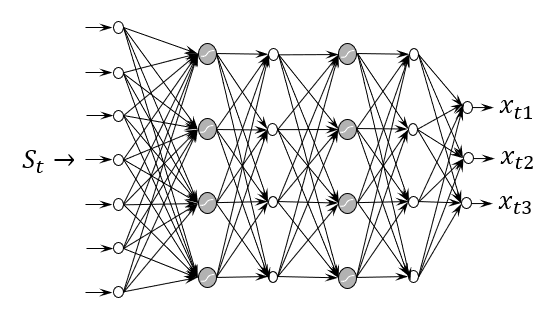
The modern (and very deep) neural networks can handle very high-dimensional state variables as input, and can produce high-dimensional vector outputs. This model was used by Amazon to plan inventories for 10,000 products — meaning $x_t$ had 10,000 dimensions — while the inputs $S_t$ consisted of any information that might be relevant in the planning of any of the 10,000 products.
Large language models
As this website was being developed (in 2026), large language models were emerging, and people realized that LLMs were very useful at guiding planning processes. What is effectively happening here is that the LLM is a form of PFA which does not have to be trained on a specific decision problem. It will offer suggestions based on the training performed in the development of the LLM. This is not a general tool that will work on any decision problem (for example, it cannot solve integer programs), it is useful for a variety of decisions, such as choosing the performance metric or even the class of policy.
Using an LLM to make a choice represents a form of type 10 decision: “deciding what to decide” — specifically, it is a decision to not perform formal analysis to determine a particular type of decision. There is nothing wrong with this, as long as there is an awareness that using an LLM to make a choice represents a case of “deciding not to decide.”