Learning while doing — the cash management game

The cash management game is an exercise in adaptively learning and making adjustments, a process we call “learning while doing.” The problem is a real application, where a mutual fund manager has to decide how much cash to keep on hand to respond to redemptions. The original motivation of the problem was revealed in an email from a mutual fund manager to a professor who taught one of his courses for his executive MBA.

The game involves trying to determine the right fraction of his assets under management to keep in cash. We start with a simpler problem where there is a single parameter to optimize, and then transition to a richer problem which involves two parameters.

This game describes a very real-world solution that can be applied to virtually any process that would benefit from adapting to conditions in the field. Players will learn about:

• Creating and updating beliefs about the process.
• Choosing among methods (“policies”) for updating tunable parameters (such as the fraction of assets to hold in cash).
• Recognizing that these policies have their own parameters.
• Understanding how noise dramatically increases the complexity of even simple problems such as this.
• Learning in the field is slow; it takes a day to observe a day.

For an introduction to the problem, watch the short video here.

Our presentation is divided into the following sections:

• The setup — a quick introduction to running the game.
• Playing the game — choose which version of the game you want to play (1 or 2 parameters), and edit the parameters that control the behavior of the game (not necessary for initial runs).
• How the game is played — a more in-depth description of how to run the game.
• Parameter adjustment policies — an overview of the methods you can test for adjusting the parameters that govern how much cash is held.
• Belief formation — an introduction to the issues that arise when creating and updating beliefs into how new information changes what we think about the performance function.

The setup

As you see from the video (which you need to watch), there are two policies for setting how much cash to keep on hand for redemptions:

• The single-parameter version — This uses a fraction (say .07) of the total cash under management.
• The two-parameter version — Use one parameter for the individual investors, and a second parameter for the institutional investors.

We would like to determine which of these two policies are best, but both have parameters that need to be tuned. To do this, we have to choose a parameter adjustment policy from the pull-down list. Finally, there is a set of advanced parameters which can be ignored for now.

“Playing the game” involves picking a value for the policy parameters (whether it is one or two). The game then simulates a number of days and reports the total performance, which is the gains from the stock market minus transaction costs.

After one batch of observations, your chosen “parameter adjustment policy” will adjust the parameters, and run another batch. You can do this as often as you like. The game will report the performance for each batch, and the cumulative performance.

You can hit restart and start over at any time.

We recommend starting with the 1-parameter policy to get a feel for the game. Note that daily performance is very noisy, so you will learn virtually nothing from running 1 or even several weeks. Part of your challenge is to determine how long you should stay with a single parameter setting before updating it (we are not going to help you pick this). Don’t be afraid to test intervals as long as 100 days, but remember — it takes 100 days to simulate 100 days in the field. This is the challenge of “learning while doing.”

Playing the game

Pick a game, then hit Play the game. Inside the game you’ll choose the parameter-adjustment policy on the control bar.

How the game is played

The game is controlled using the settings in the control bar that looks like:

The game starts by choosing initial values of the cash management parameters in the Starting point box. You might choose 0.10 for the single-parameter version, or (0.10, 0.10) for the two-parameter version.

The system then simulates a number of days set in the Run box. If this box is set to 50, then it will simulate 50 days using the initial values for the policy parameters.

The next pulldown menu provides a set of choices for the policy used to update the policy parameters. These parameter settings are only used in the next batch of simulations (e.g. the next 50 days).

The Repeat box will repeat the process of updating the parameters, and simulating the next batch of days. If this is 0, then the model does a single simulation of the batch (50 days) and stops. The Starting point box will update to Current point and show the value that will be simulated if you perform another batch by hitting the button One more.

After hitting the Run button, you might see something like:

You can keep doing one more batch at a time by hitting One more (as long as Repeat is set to 0). If you set Repeat to 10, it will run another batch and update the parameters 10 times using the specified parameter-adjustment policy. The points that are selected at the end of each batch are shown in the graphic below.

If you hit Restart it resets the game to the starting points, and zeroes out the boxes reporting the performance and number of days.

Parameter adjustment policies

To determine how to adjust the parameter policies $\theta$, we need some method. Below, we review two simplistic policies (manual and random), along with the two policies reviewed in the video above: interval estimation, and a family of policies based on the concept of the knowledge gradient which is based on the value of information obtained from observing performance over a period of time.

Manual policies

A manual policy requires a human (you) to review the behavior of the system and make a subjective adjustment of what to try. Go ahead and try to compete against the other policies (don’t laugh — you may win!).

Randomized policies

A popular class of policies in the reinforcement learning literature is to introduce randomization. A purely random policy makes no sense for an online setting, we could use a mixture of doing what we think is best based on our current (but imperfect) belief, and something random that we test just for learning.

The challenge in this setting is handling the high level of noise when we try any policy, regardless of whether we think it is best or we are exploring something different.

Interval estimation policies

An IE policy is written

where $\mu_{\theta}^{n}$ is the current estimate of the performance of the cash management parameter $\theta = \theta^{cash}$. The variable $S^{n}$ captures our “state of knowledge” about how well the system performs after $n$ updates. The policy parameter $\rho^{IE}$ also has to be tuned, which means we are tuning a parameter in the policy $\Theta^{cash}!\left(S_{t} \mid \rho^{IE}\right)$ that is used to tune the parameters in the cash management policy.

One way to compare the parameter $\rho^{IE}$ is to test different values over a range. It is likely that $\rho^{IE}$ will fall in the range $[0, 3]$, which helps with the process. Testing values in increments of 0.2 is one approach to find the best value of $\rho^{IE}$.

Knowledge gradient policies

The “knowledge gradient” (or KG) is a policy that estimates the value of information from an experiment. This means estimating how much better future decisions will perform after watching the performance of some value of $\theta^{cash}$ for a period of time (such as 50 weeks). See below for more information about the knowledge gradient.

Choosing how long to observe the process is its own parameter. If it is too short (say a week) then what you are going to observe is sheer noise, and you will not learn anything (imagine trying to decide how much auto insurance to have based on what happened last week). You might learn much more if you choose 50 weeks, but this means waiting an entire year before taking advantage of what you have learned. Playing with this parameter is one of the goals of the game.

Knowledge gradient policies come in two flavors:

• Offline knowledge gradient — This computes the value of information completely ignoring the actual performance. For example, we might try holding only 1 percent of cash reserves. Let $KG^{offline}(\theta^{cash}; \rho^{lkhd})$ where $\rho^{lkhd}$ is called the “lookahead parameter” which is an integer giving how many days the knowledge gradient peeks into the future to calculate benefits. The best value for $\rho^{lkhd}$ depends on how noisy the simulations are. We might use $\rho^{lkhd} = 1$ for low-noise simulations, and $\rho^{lkhd} = 50$ (or more) for higher-noise problems.
• Online knowledge gradient — Here we balance our current estimate of how well our system is performing (which might be completely off) against the value of the improved performance that we might obtain if we test a policy now. This introduces a new twist: how long should we assume we are going to benefit from the information we just gained? This is an important tradeoff that you will have to explore in the game.

The online knowledge gradient is computed using

Here, $\mu_{\theta}^{n}$ captures our current (possibly incorrect) estimate of the performance of our cash management policy using $\theta^{cash} = \theta$.

For readers who would like a more in-depth treatment of the knowledge gradient, see the material on the optimal learning webpage.

How the knowledge gradient works

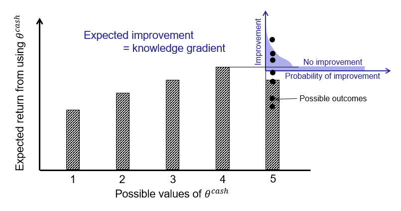
The knowledge gradient was introduced by Peter Frazier in 2007 for offline learning problems, and later extended by Ilya Ryzhov to online learning. The logic behind the knowledge gradient is described in the video introducing the cash management game above, but a quick explanation uses the graphic to the right (from the video).

Imagine we have five possible values of the parameter $\theta^{cash}$ that we are trying to optimize. Also imagine we have imperfect estimates, but for now we think the fourth value is best. We want to estimate the value of the information we would obtain if we tested the fifth value.

If we test the fifth value, and update our estimate of its performance, we only benefit if the updated estimate of the performance is better than what we currently estimate for the fourth value. If this is not the case, then we still think the fourth value is best, which means testing the fifth value does not change our decision of which of the five values is best.

If we did many simulations using the fifth value of $\theta^{cash}$ (using our simulator), we might obtain any of the black dots. Some of these are improvements that would increase our estimate of the fifth value, while others would not. If we performed many of these simulations, we could build a probability distribution of the updated estimate of the fifth value.

There is a probability that the improvement is zero (shown as a big spike), and then there are probabilities that testing the fifth choice is an improvement. The knowledge gradient, then, is the expected increase in the value of the best choice.

For an in-depth technical presentation of the knowledge gradient, see the optimal learning page (see the sections that refer to “knowledge gradient”).

Belief formation

(section content to come)