Multiagent modeling

There are countless settings involving making decisions, where it makes sense to divide the system into agents performing different functions. This is most vividly illustrated when modeling a spatially distributed supply chain where people are making decisions around the world which have to be coordinated.

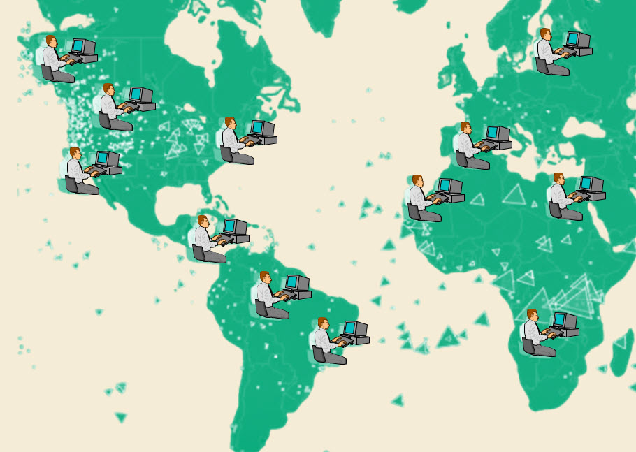
Even the most basic sequential decision problem is best viewed as consisting of two agents: 1) the environment, which knows the ground truth about underlying process governing the evolution of systems over time, and the generators of new information, and 2) a controlling agent that makes decisions that affect the evolution of the system in some way.

All the material in this section is based on Chapter 20 of Reinforcement Learning and Stochastic Optimization. Chapter 20 can be downloaded here. The discussions below represent a high-level tour of this chapter.

Jump to a section

• Types and capabilities of agents
• From stochastic optimization to a two-agent model
• The POMDP formulation
• Multiagent notation
• Modeling: From single to multiple agents
• Examples of multiagent problems

Types and capabilities of agents

The term “agent” can be applied to literally hundreds of settings, spanning people, devices, machinery, robots, computer software, and companies. We start by providing a list of the types of agents along with their capabilities:

1. The environment — This agent holds the ground truth of quantities, parameters and processes that determine how the system evolves over time, and the creation of exogenous information.
2. Decision-making/controlling agents — These are the agents that control quantities, parameters and processes that govern the evolution of the system. These agents may be a piece of software, a person, a group or an organization.
3. Data repository — An agent may accept data from external sources, and share it on request.
4. Observation and learning — These agents may make observations (testing patients, observing inventories) and perform learning to estimate quantities and parameters that cannot be observed perfectly.
5. Communication — One agent may send or share information with other agents.
6. Resource agents — These can serve as suppliers and/or consumers of physical or financial resources.
7. Physical agents move or operate equipment (people, trucks, robots, machines, drones, generators) or control a physical system (heating and air conditioning, dams, health monitors). Physical agents typically act on the instructions from a decision-agent, but they may combine decision-making and implementation as happens with people (equipment operators), autonomous systems (intelligent HVAC systems), and robots.

The structure of a multiagent system is determined by specifying:

1. Number and type of agents — We may have: a. A single controlling agent interacting with the environment. b. Two agents who may be competitive or semi-cooperative. c. Arbitrary sets of cooperating and/or competitive agents.
2. Coordination mechanisms — Are each of the agents behaving completely independently, or is there an overarching controlling mechanism?
3. Communication architecture — This determines who can communicate with whom.
4. Reward structure — Which agents are rewarded, and how. This determines the degree to which agents are cooperative or competitive.
5. Resources — Agents often have to manage resources. A common example is energy which agents need for propulsion, but an agent may be distributing vaccines, medical supplies, ammunition, food, water, parts, etc. We would need to specify: a. Which resources does an agent need to manage? b. How much of the resource can the agent can store? How much is consumed by the agent itself? c. What are the exogenous demands that have to be satisfied (and how are these learned)? d. How is it replenished (does it return to a home base, refilling stations, or can it be visited by replenishment agents)?

From stochastic optimization to a two-agent model

Sequential decision problems are driven by two processes, decisions (which is the information we control) and an exogenous information process, which arrives from outside the system and affects how the system performs. A natural way of viewing this system is one consisting of two agents:

• The environment, which knows the truth driving all exogenous information processes.
• The decisions, made by a decision maker (or controller). The performance of the system after the decision is made depends on the information that arrives from the environment.

Recognizing that these two processes can be modeled as “agents” seems fairly straightforward. We can model exogenous information as samples from distributions known only to the environment agent, with decisions coming from the controlling agent. In fact, this perspective is not used in any book on stochastic optimization. Even my own book, Reinforcement Learning and Stochastic Optimization, published in 2022, does not mention multiagent models until chapter 20.

It is fairly common (but not universally so) that stochastic optimization problems assume the underlying probability distributions driving a stochastic process are known. This would never be true if we represent uncertainties as coming from an environment agent, since we would have to explicitly model who knows the distribution and how this information is shared. The controlling agent would never know the underlying distributions — it only has access to observations from the environment.

A more subtle assumption often made in stochastic models is that the functions driving an underlying physical are known, whether it is a physical process or the process of updating beliefs. This might be reasonable if the physics are generally known, such as how inventories are updated, the speed at which a vehicle moves, or how beliefs are updated using recursive learning. However, imagine modeling the spread of disease through a population, or the spread of information about a new product. Both of these are physical processes where the equations describing the physics would not be known to a decision-maker.

The POMDP formulation (section 20.3 in RLSO)

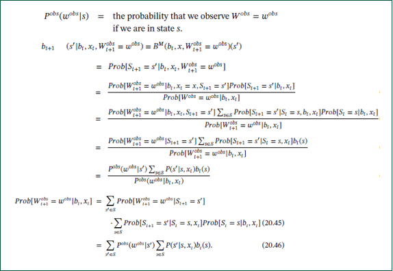While there is an extensive literature on multi-agent systems, the only formal framework addressing the identification of optimal decisions in the context of a single decision-maker and an uncertain environment is known as “partially observable Markov decision processes,” popularly known as “POMDPs.”

While POMDPs have been very popular with the probability community, they have seen little in the way of practical applications. The underlying theory requires an intense exercise using Bayes theorem that is computationally intractable for the complex state variables that actually arise in practice. It depends on Bellman’s equation for making decisions, which has its own computational challenges.

Ultimately, after all this theory, the results do not scale computationally, and they would never be optimal a) because Bellman’s equation cannot be computed and b) because of the various modeling approximations that are being made.

Multiagent notation

We start with a brief review of our single-agent notation, and then show how to extend it to multiple agents.

Single agent notation reviewed

We have been modeling sequential decision problems using the following notation:

$S_{t} =$ Our state of knowledge at time $t$ which consists of:

$R_{t} =$ Quantities of resources of different types at time $t$. We might let $R_{ta}$ be the number of resources with attribute $a$ at time $t$, where $a$ may be a vector.

$I_{t} =$ Information about parameters and functions at time $t$.

$B_{t} =$ Beliefs stored about any uncertain quantities and parameters that we do not know perfectly. Beliefs may be stored with a mixture of frequentist or Bayesian statistics.

$x_{t} =$ A (possibly vector-valued) set of decisions that act on our system in any way, whether it is changing quantities, parameters, or functions that affect the evolution of the system.

$W_{t+1,i} =$ The information of type $i \in \mathcal{I}^{\inf}$ which arrives after decision $x_{t}$ is made, and before we make decision $x_{t+1}$. Information may arrive from a variety of sources over different time scales.

Our state variable evolves according to the state transition model:

which covers the updating of quantities of resources $R_{t}$, information about parameters (and possibly functions) $I_{t}$, and beliefs $B_{t}$ about quantities and parameters that we only know with uncertainty.

Extension to multiple agents

We start by introducing our index for agents:

$q \in \mathcal{Q} =$ A (finite) set of agents.

We reserve $q = 0$ for the environment, which occupies a special place in our multiagent vocabulary. If we work on a two-agent problem, we suggest letting “0” be “agent 0” for the environment, and then letting “$q$” (which is a letter, not an index of a set) as our decision-making agent.

If we have multiple decision-making agents, we might use $q_{1}, \ldots, q_{\lvert\mathcal{Q}\rvert}$ to label each agent, or simply let $q \in {0, 1, 2, \ldots, \lvert\mathcal{Q}\rvert}$ be the indices for each agent, where we reserve $q = 0$ for the environment.

Once we establish our “$q$” notation for agents, we can model our state variable as

where we always let time $t$ be the first index so that we can write the state of our system as

The decision vector would be $x_{tq}$ and the exogenous information arriving to agent $q$ would be $W_{t+1,q,i}$.

To create a compact canonical model, we need to realize that the decision vector $x_{tq}$ has to represent any decision, whether it is the flow of resources, parameter settings, or choice of functions. For our multiagent problem, it also has to represent the decision to send information (a type 4 decision) or observe a process (a type 3 decision). By the same token, $W_{t+1,q,i}$ may be the arrival of new customer requests, changes in prices, or what we learn about a patient from an MRI. $W_{t+1,q,i}$ may also be an observation of a decision by another agent, which allows us to update our beliefs about their behavior (more on this below).

Our transition function would be written

We need to emphasize how much we are hiding in this single equation. It covers updating the status of physical resources, changes in what we know about parameters and functions, and the updating of beliefs about any quantities and parameters that we do not know perfectly.

Beliefs about the state of other agents

A major change when we extend to multiple decision-making agents is the need to represent what other agents know. We use the notation

$S_{tqq’} =$ The state of what agent $q$ knows about agent $q’$ at time $t$.

Examples of this kind of information include:

• The amount of inventory on hand at a supplier $q’$ that is estimated (but not known perfectly) by the manufacturer $q$.
• The type of policy that agent $q’$ is using to make decisions, which would allow agent $q$ to anticipate how $q’$ might react.
• Whether a patient $q’$ is dieting so that the physician $q$ can understand how it might be affecting their health.

From big systems to sets of small systems

Our multiagent notation lays the foundation for a full multiagent system. In the process, it highlights the generality of our original notation. For example, return to the multiagent supply chain that we illustrated at the top of the section. Instead of having a very high-dimensional state variable $S_{t}$ that describes the status of every single manufacturer spread around the world, we would model each individual manufacturer as a separate agent, which more accurately captures how the system might be managed.

A multiagent model is illustrated below. Each box captures the scope of a single agent which might be the manager of a single manufacturing plant, or a scientist running a lab, or a physician in the field.

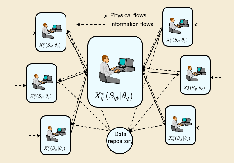
The dashed lines in the figure indicate the flow of information, which may be to or from a data repository. Solid lines represent the flows of physical or financial resources.

Modeling: From single to multiple agents

We have shown how we can leverage our single-agent notation to model multiple agents, but this hides the richness of the multiagent setting. For example, while belief state variables arise often in a single-agent setting, seeing them in actual models is quite rare. They are non-existent in deterministic optimization models, but stochastic, dynamic models that explicitly model a belief state are hard to find.

This situation changes dramatically when we transition to multiple agents. Even a two agent model, consisting of a decision-maker and environment, requires that the decision maker construct a belief about the environment.

When we transition to multiple decision-makers, we introduce the dimension of learning about the behavior of the other decision makers, which is the same as saying that we are learning about the policies they use for making decisions. Learning behaviors when we have adversarial agents is critical. There is a vast literature of stochastic, dynamic problems which do not explicitly model belief state variables (see for example any book on Markov decision processes).

Physical flows between agents

There are many settings, with supply chain management being the most visible, where one agent can send physical resources (parts, products, people, water, chemicals, money) to another agent. To represent this, we introduce the notation:

$\mathcal{Q}_{q}^{+} =$ Set of agents $q’$ that an agent $q$ can send physical resources to.

$x_{tqq’a} =$ Flow of resources with attribute vector $a$ from $q$ to $q’$ at time $t$ (there may be some lag before the resources arrive at agent $q’$). We can use this notation to represent any action by agent $q$ on agent $q’$ at time $t$.

There is a lot of other notation required to fill out the dynamics that can be found in chapter 20, but this provides a start.

Travel times

When we move physical resources, we have to recognize that transportation takes time. We cannot say that a movement initiated at time $t$ will arrive at time $t + 1$. If a supply chain model is using a day as a time step, ordering production from the far east might require 40 to 160 days (or more).

In a deterministic model, transitioning from single to multiperiod travel times does not have a big impact on the model. However, if we have a fully sequential decision problem where we are modeling the arrival of estimation, multiperiod travel times can introduce a significant source of complexity.

We cannot, for example, simply assume that transportation times follow some distribution, where we have to sample the travel time from the distribution. Delays arise during the course of the trip, from being released at origin (reflecting the manufacture of the part), to delays at ports, weather delays, and equipment problems (to name a few). In our multiagent system, we not only have to model what delays happen, but also who knows this information, and what is communicated to other agents.

Information flows between agents

Easily the most subtle dimension of modeling multiagent systems is capturing the flow of information between agents, where this may consist of information that agent $q$ sends to $q’$, or information agent $q$ receives from $q’$, either because the information was sent by $q’$, or agent $q$ was able to make an observation without any explicit action by $q’$.

Given the subtleties of sending and sharing information, it helps to introduce new notation rather than re-using our “$x_{tqq’}$” notation. We can define:

$z_{tqq’i} =$ The sharing of information from element “$i$” known to agent $q$ with agent $q’$ at time $t$.

If you are agent $q’$, you are told that $z_{tqq’i}$ is informing you about information held by agent $q$ at time $t$. This might be the status of a production line, a patient reporting on their condition, the status of a piece of equipment, or the location of a shipment. However, the information may not be accurate. We might need to capture:

$\beta_{qq’i} =$ The precision (inverse of the variance) of the reliability of the information sent from $q$ to $q’$ describing information element $i$.

$\delta_{qq’i} =$ The bias in the information about data element $i$ sent from $q$ to $q’$.

Bias and variance (precision) are two key statistics capturing the reliability of information. It is very common that information arrives with errors, which may consist of bias (being consistently high or low) plus noise, captured by the variance. These parameters can reflect the relationship between $q$ and $q’$ (we are more honest with some people than others).

We are typically aware that it costs money to move physical goods from one agent to another, while moving information is often negligible. This is not the case, for example, when we are dealing with robots/drones, so we might also capture:

$\eta_{qq’i} =$ The energy required to send information about data element $i$ from $q$ to $q’$.

Energy consumption is an important consideration for robots and drones, hence the energy requirements for communication need to be considered.

Exogenous information as exogenous decisions

The most standard notation for sequential decision problems is to represent the information arriving after we make a decision $x_{t}$ as $W_{t+1}$, which is illustrated using processes such as rainfall, equipment failures, customer demands and market prices, with the implicit assumption that our decisions do not affect the market.

In fact, there are so many problems where an exogenous input is the result of decisions of external agents, for example:

• A doctor has to decide on the treatment of a patient while dealing with decisions by the patient on following instructions.
• A grid operator has to plan which generators to use tomorrow, which is subject to decisions of the operator of the generator that affect compliance.
• A financial planner has to work with whether a customer follows their investment recommendations.

An exogenous agent does not have to be an individual — it can be a market representing the collective decisions of many people. As a result, a pricing decision can affect demand for a product, while a decision to sell a large block of stock can depress prices.

The ability to influence exogenous information processes is common, which is why I started to write the exogenous information process as a function:

$W_{t+1,i}(S_{t}, x_{t}) =$ Information of type $i$ arriving between $t$ (that is, after we make decision $x_{t}$) and $t+1$ (before we make decision $x_{t+1}$), which might be influenced by the current state $S_{t}$ (that is, what we know before we make decision $x_{t}$) and/or the decision itself $x_{t}$.

It is usually the case (but not always) that the state $S_{t}$ reflects previous decisions. As a result, dependence on either $S_{t}$ and/or $x_{t}$ implies that there is another agent (or group of agents) that is making its own decisions that affects the information arriving to the agent making the decision $x_{t}$.

Examples of multiagent problems

There are countless examples of multiagent problems. In fact, all sequential decision problems can (and probably should) be viewed as multiagent problems, such as an environment agent and a decision agent. However, the vast majority of decision models are simply models of a particular decision maker in the presence of other decision makers. In this section we are going to cover:

• A flu mitigation problem
• The two-agent newsvendor problem
• The beer game

A flu mitigation problem (section 20.2 in RLSO)

Section 20.2 describes a series of variations of a problem of mitigating the spread of the flu, where the status of the flu is treated as the environment. The decision agent controls how vaccines are distributed and the guidelines for their use.

A major dimension of the problem is the process of modeling how the flu spreads within the population. We start by writing out a complicated function that is known only to the environment, which describes how the true mean rate of infection, given by $\mu_{t}$ at time $t$, evolves over time:

where $U_{t-1}$ and $U_{t-2}$ are functions that capture how cold it is relative to a reference temperature (where people start coughing more). The structure of this function is not important, other than to make the point that it is complicated, and unknown to us.

Given that we do not know the true process governing the spread of the flu, we are going to make up a simpler time series model that captures what we think are the important explanatory variables. Assume that this exercise produced the following model:

The point of making up the first transition function is to emphasize the idea that there is some true function that we don’t know and can’t guess. Instead, we make up a simpler model that we think will capture the important behaviors.

The first function is known to the environment, while the second is one known to the controller, who now faces the problem of estimating the vector of coefficients $\theta$ from whatever we can observe.

A common mistake is to start with the second model above, assume the structure of the function is correct, and then assume that the only error is that we do not know the precise values of the coefficients $\theta$. The difference between the two models is well known in economics (where the field is called econometrics), where it is called specification errors.

This little exercise highlights the difference in perspectives when we adopt the perspective that anything uncertain comes from a different agent (such as the environment), which may mean that not only do we not know the values of parameters, we may not know the underlying function itself. We refer the reader to section 20.2 of RLSO for a more in-depth discussion of this model.

The two-agent newsvendor problem (Section 20.4 of RLSO)

The newsvendor problem is one of the oldest problems in operations research, where we place an order for product and then observe the demand. The simplest model assumes the distribution is known, but the more interesting case (which has been studied since the 1950s) is where the distribution is unknown and has to be learned.

And then there is the two-agent version, which describes most real-world settings. The original newsvendor assumes that if you request $x$ units of product (the “newspapers”), you get $x$. In the two-agent variant, we assume there is a field agent, who we will call $q$, who directly faces the market demand, and a central agent, who we will call $q’$, who allocates resources. The field agent places a request $x_{tqq’}$ on day $t$ to the central agent $q’$.

The central agent $q’$ wants the field agent to do well, but each agent has their own cost of having too many (overage) or too few (underage). The field agent faces the market, and as a result has a strong aversion to not being able to satisfy demand. The central agent has a more balanced attitude toward unsatisfied demand versus having excess inventory left over (which has to be discarded).

This means that while the two agents are presumably working for the same company, they each have their own objective function.

The image below describes the flow of information on each day, where the field agent is assumed to be able to see information that provides a hint about that day’s demand. His request is then transmitted to the central agent who balances this request against other sources of information, including historical knowledge. The central agent then solves her own decision problem, which assumes a balanced attitude toward uncovered demand and excess inventory.

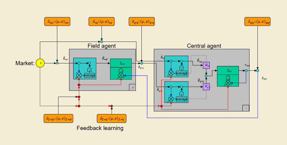
If this were a single agent problem, the field agent would ask for more than he needs, because he assesses a high penalty for unsatisfied demand. Because the central agent does not share this bias, she is typically reducing his request, and the field agent knows this, so he inflates his original request to compensate for an anticipated reduction. The central agent, of course, knows that the field agent is doing this, and compensates accordingly.

This model (described in much more detail in section 20.4 of Reinforcement Learning and Stochastic Optimization, but also see Chapter 10 of Sequential Decision Analytics and Modeling), introduces a nice example of learning about the behavior of other decision-making agents. This opens up new opportunities for designing policies. Consider the following (assume we are the field agent, but everything applies to the central agent):

1. The field agent makes the best decision he can given his current belief about how much the central agent might reduce his request. This means the field agent is inflating his request to compensate for the anticipated reduction that the central agent will impose. However, the field agent ignores how his behavior will change the behavior of the central agent.
2. The field agent begins with the strategy of (1) above but recognizes that the central agent is going to adjust her own behavior after seeing his request. He now anticipates how his request will change the behavior of the central agent and adjusts his behavior accordingly. This will have the effect of encouraging him to be less aggressive in his requests so that the central agent will be less aggressive in her requests.
3. The field agent adjusts the strategy of (2) by realizing that the central agent may also be anticipating how her decisions may change the behavior of the field agent.

In other words, the behavior of one agent can (and should) recognize how the behavior of the first agent changes the behavior of other agents. While this level of sophistication seems unlikely in the negotiations of the level of resources to allocate to field personnel, the same issues arise when large chemical manufacturers are bidding for very large projects in an oligopolistic market which consists of only two or three players.

The beer game (Chapter 11, Sequential Decision Analytics and Modeling)

The beer game was developed by Jay Forrester at MIT in the 1950s and has grown into a standard exercise in supply chain management classes. It consists of at least four “echelons” where beer is moved from the factory through several states of storage and distribution before meeting the demands at a retailer.

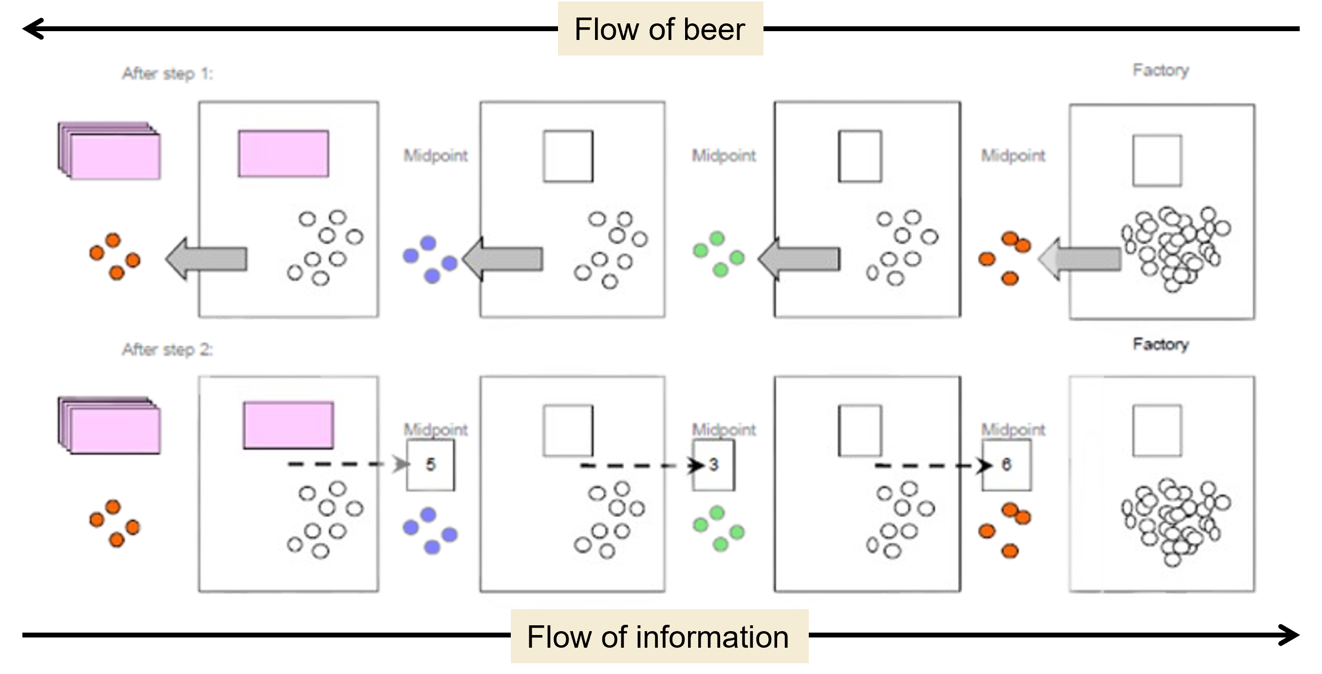
Beer (top line) moves from right to left, usually in the form of pennies (as the game is played). The amount of beer is determined by requests that are written on slips of paper that are moved from left to right (bottom line), nicely capturing both the flows of physical goods (cases of beer) and information (the requests). The game does not model cash flows and financing.

Each echelon is a separate agent who receives orders from the left and tries to satisfy them. If an echelon does not have enough beer to meet an order, the unsatisfied orders are stored in a backlog, which incurs additional penalties.

In theory the echelons are not allowed to communicate, which means that the state variable for each echelon consists of their current inventories and backlogs, along with the histories of previous orders from the upstream echelons (or market), back orders that have not been received yet, and the history of orders received which an echelon can relate to the orders they have placed.

This problem could be solved using any of the four classes of policies, but PFAs (policy function approximations) are the most widely studied as a teaching exercise. Section 11.6 of Sequential Decision Analytics and Modeling presents a series of “anchor and adjustment” policies using the principles proposed by the renowned decision psychologists Daniel Kahneman and Amos Tversky.

To illustrate an anchor-and-adjustment policy, first define:

$\bar{F}_{t,q-1,q} =$ Estimated fill rate to agent $q-1$ by agent $q$ ($q-1$ is one echelon closer to the retailer $q$).

$\bar{A}_{t,q-1,q} =$ Actual beer orders from agent $q-1$ to agent $q$.

There are different ways to compute $\bar{F}_{t,q-1,q}$; one, called “adaptive estimation” is given by

Next define:

$\delta R_{tq}^{inv} =$ Adjustment based on the current inventory $R_{tq}^{inv}$.

$\delta R_{tq}^{transit} =$ Adjustment based on the current in-transit inventory $R_{tq}^{transit}$.

These quantities might be estimated using

where $R_{q}^{inv - trgt}$ is a target inventory for agent $q$, while $R_{tq}^{inv}$ is the current inventory. $\delta R_{tq}^{transit}$ can be calculated similarly for the amount of inventory that is in-transit.

A type of anchor-and-adjustment policy is then given by

Variations of this and another policies are given in section 11.6 of Sequential Decision Analytics and Modeling.

It is possible to envision using any of the four classes of policies for the beer game. Anchor-and-adjustment attracted attention because of its simplicity, although the tuning process has been largely overlooked. However, real supply chain planning would always have to use some form of direct lookahead approximation; a version of a DLA is given in chapter 20 of RLSO.