Chapter 5: Uncertainties
Sequential decision problems invariably have to deal with uncertainty, which is typically the most challenging dimension of making decisions over time. There are three ways that uncertainty affects the performance of our system:
- The decision we make at a point in time is not implemented correctly.
- The performance of the system given our decision is not the same as what we estimated when we made the decision.
- The impact of a decision now on the future is not estimated correctly because of changes as we step forward in time.
Although we list only three ways that uncertainty affects performance, uncertainty arises in many forms, which is why some forms of uncertainty are often overlooked in the modeling process. In fact, most uses of optimization tools ignore all forms of uncertainty, typically reflecting the dramatic increase in uncertainty introduced by explicitly modeling any form of uncertainty.
A goal of this chapter is to highlight the different ways that uncertainty can arise. This does not mean that models need to incorporate all forms of uncertainty. However, the decision to ignore a form of uncertainty should be an explicit choice, and not just because a modeler overlooked it.
The 12 classes of uncertainty {#12classesofuncertainty}
One way to approach the identification of sources of uncertainty is to work backward from a mathematical model. Below are 12 classes of uncertainty created from the perspective of how uncertainty can enter a model. Complex problems, such as managing a supply chain, an energy system or solving a public health problem, will involve all 12 classes, while simple problems such as playing chess may involve just one.
There is some overlap in the classes, so do not worry if there is some ambiguity in terms of where to list a source of uncertainty. What is important is to identify as many different forms of uncertainty as possible.
- Observational errors – These represent errors in quantities and parameters that we have to observe from the environment. Some examples might be:
- The current inventory of a product as represented in the computer, which may not match what is actually on hand.
- Medical X-rays of a patient to detect cancer.
- The fraction of voters who prefer a particular candidate for political office.
- Exogenous uncertainty – This is information that will arrive to our system after making a decision, such as:
- The demand for a product being sold in the market.
- The change in price of a stock.
- The time required to drive from one city to the next.
- The amount of cash that may be deposited or withdrawn tomorrow.
- How a patient responds to a type of medication.
- Prognostic uncertainty – This is errors in forecasts of demands, prices, travel times (any quantity that we might be forecasting).
- Inferential uncertainty – This captures uncertainty in our estimates of the state of the world right now. This could include:
- How the market might respond to a change in price. We might think there is a 10 percent drop in demand for a 5 percent increase in price, but the true value might be that demand will drop by 12 percent.
- We think that a cancer patient is stage 2, but it might be stage 3. We might detect breast cancer, but overlook that it has spread to other organs.
- A presidential campaign may think that $10 million in ad spending in a major market might produce a 2 percent increase in favorability of a candidate, but the reality may be higher or lower.
- Experimental uncertainty – This describes the variation from running repeated experiments either in a lab, a simulator, or the field:
- A manufacturer runs experiments of a process for manufacturing silicon wafers. The test may be repeated 10 times, producing a spread of yields between 70 and 90 percent.
- A business is evaluating a new marketing campaign by running it in five different test markets. There will be variations across the markets, and over time.
- A computer simulator is used to test the performance of an inventory ordering policy. Each pass of the simulator will produce different results.
- Model uncertainty – This is an umbrella that can cover multiple sources of uncertainty, but one of the most important is uncertainty in the model of how a process evolves over time. Examples might be:
- How the climate responds to changes in policies for controlling carbon.
- How a patient responds to injections of insulin.
- How a disease spreads in a population in response to changes in policies regarding the distribution of vaccines.
- Transitional uncertainty – This is noise in how a system responds to a control. The simplest example would be controlling the path of a rocket or aircraft, which is buffeted by wind. We typically assume that the evolution of the system is known and deterministic, but is affected by an exogenous process (such as wind).
- Implementation uncertainty – There can be a difference between what we decide to do, and the decision that is actually implemented in the field. For example:
- The physician orders a particular medication, but the patient does not take it, or takes the wrong dose.
- A scientist wants to test a particular combination of materials, but the intern orders an incorrect item (errors like this can produce major breakthroughs!).
- The power grid orders that a generator be turned on at 1pm, but the local operator does not turn on the generator until 2pm.
- Communication errors – Instructions to the field can be simply miscommunicated. The person receiving the instruction may think they are doing what is requested, but they just did not hear or understand an instruction.
- Algorithmic instability – There are some settings where running an algorithm repeatedly can return different solutions:
- Complex problems often require the use of sophisticated algorithms that introduce an element of variability, which often arises when an algorithm uses parallel processing. The speed of parallel processors may affect who finishes first, which can affect the overall path of the algorithm.
- Algorithms for solving stochastic optimization problems often depend on Monte Carlo sampling which will produce different results each time the algorithm is run (this is seen when running large language models).
- Goal uncertainty – Companies that require groups of people to make decisions (dispatching trucks, trading financial assets, bidding on energy contracts) can exhibit variations because different people emphasize different performance metrics.
- Environmental uncertainty – Here, “environment” might reflect climate, or a political environment (which might impact policies or tariffs), or new management at a company (which results in a change in priorities).
Examples from selected applications
It helps to see examples of each of the 12 classes for some of the applications we introduced in Chapter 2. For each application, we describe one or more examples of the uncertainties for each class, noting that simpler applications will not have uncertainties for all 12 classes. It is important to remember that the real goal here is to recognize as many sources of uncertainty as possible. How these uncertainties are reflected in the process of making decisions will come in future volumes.
Cash management for a mutual fund
A mutual fund has to determine how much cash to keep on hand to meet redemption requests, and as deposits are made, by both individual and institutional investors.
| Classes of uncertainty | Mutual fund cash balance |
|---|---|
| 1. Observational uncertainty | |
| 2. Exogenous uncertainty | Deposits, redemptions, market indices |
| 3. Prognostic uncertainty | Forecasts of deposits, redemptions, market indices, interest rates |
| 4. Inferential uncertainty | Estimating how redemptions change with market performance |
| 5. Experimental variability | Testing different policies for holding cash |
| 6. Model uncertainty | |
| 7. Transitional uncertainty | Updating how much cash is on hand |
| 8. Implementation uncertainty | |
| 9. Communication errors | |
| 10. Algorithmic instability | |
| 11. Goal uncertainty | Balancing maximizing investment returns, minimizing stock sales for redemptions |
| 12. Environmental uncertainty | Changes in interest rates |
Finding the best diabetes treatment
Diabetes patients have to manage their blood sugar using a combination of medications (perhaps using an insulin pump) and diet.
| Classes of uncertainty | Managing blood sugar |
|---|---|
| Observational uncertainty | Measuring A1c levels |
| Exogenous uncertainty | What a patient eats |
| Prognostic uncertainty | Anticipating changes in blood sugar levels after a meal |
| Inferential uncertainty | Estimating how a patient's blood sugar responds to medication |
| Experimental variability | Changes in blood sugar for different types of medication |
| Model uncertainty | Modeling how a patient responds to a type of medication |
| Transitional uncertainty | |
| Implementation uncertainty | Whether a patient follows their physician's instructions |
| Communication errors | Whether a patient misunderstands the physician's instructions |
| Algorithmic instability | |
| Goal uncertainty | Balancing blood sugar reduction vs. digestion issues |
| Environmental uncertainty |
Supply chain management
Supply chains require managing inventories that have to be coordinated across the system.
| Classes of uncertainty | Supply chain management |
|---|---|
| 1. Observational uncertainty | Measuring inventory |
| 2. Exogenous uncertainty | Market demand, weather, transit times |
| 3. Prognostic uncertainty | Forecasting demands, production, resignations |
| 4. Inferential uncertainty | Market response to price, machine failure rates |
| 5. Experimental variability | Simulation errors, testing new materials, test marketing |
| 6. Model uncertainty | How information spreads in the marketplace, how employees respond to incentives |
| 7. Transitional uncertainty | Updating inventories |
| 8. Implementation uncertainty | Failure to follow instructions |
| 9. Communication errors | Incorrect instructions to suppliers |
| 10. Algorithmic instability | Variations in optimal solution from production schedules |
| 11. Goal uncertainty | Differences in priorities toward production cost vs. covering demand |
| 12. Environmental uncertainty | Changes in tariffs, currency exchange rates, interest rates |
Allocating naloxone kits
State agencies have to allocate naloxone kits to meet the needs of local clinics and medical professionals who are treating patients.
| Classes of uncertainty | Management of naloxone kits |
|---|---|
| Observational uncertainty | The number of naloxone kits in inventory |
| Exogenous uncertainty | The number of events requiring uses of naloxone kits |
| Prognostic uncertainty | Estimates of changes in patterns of drug use |
| Inferential uncertainty | Estimates of how the availability of kits affects their use |
| Experimental variability | |
| Model uncertainty | Understanding how drug use patterns change over time |
| Transitional uncertainty | Changes in naloxone kit inventories from week to week |
| Implementation uncertainty | Whether kits are used properly; whether instructions to allocate are followed |
| Communication errors | Whether field representatives follow instructions in handing out kits |
| Algorithmic instability | |
| Goal uncertainty | Prioritizing who to supply with naloxone kits |
| Environmental uncertainty | Availability of funding for naloxone kits |
Managing a fleet of trucks
Truckload trucking companies have to determine which loads to move, with what driver.
| Classes of uncertainty | Managing a fleet of trucks |
|---|---|
| Observational uncertainty | |
| Exogenous uncertainty | New loads from shippers; refused assignments by drivers; traffic delays |
| Prognostic uncertainty | Forecasts of loads in the future |
| Inferential uncertainty | How the market will respond to changes in spot prices |
| Experimental variability | Running simulations of changes in driver allocations |
| Model uncertainty | |
| Transitional uncertainty | Changes in number of available loads; updates to driver availability |
| Implementation uncertainty | Whether a dispatcher follows the instruction of the model |
| Communication errors | Whether dispatchers follow the instructions of their managers |
| Algorithmic instability | Changes in the solution from updates of estimates of driver values |
| Goal uncertainty | Balancing empty miles against shipper commitments against getting drivers home |
| Environmental uncertainty | Changes in hours-of-service rules by the Dept. of Transportation |
Planning an electric power grid
The power grid has to work with utilities to determine which generators should be turned on to meet the anticipated demands placed on the grid.
| Classes of uncertainty | Managing the electric power grid |
|---|---|
| Observational uncertainty | Estimating temperature, weather, customer attitudes |
| Exogenous uncertainty | Changes in weather, generator failures |
| Prognostic uncertainty | Forecasts in temperature, wind, cloud cover |
| Inferential uncertainty | Estimating how power demand changes as grid prices change |
| Experimental variability | Variability in the response to changes in model parameters |
| Model uncertainty | Errors in evolution of wind speeds over geographical region |
| Transitional uncertainty | Difference between expected wind power and actual |
| Implementation uncertainty | Differences between instructions to utilities and what they do |
| Communication errors | Errors in understanding of instructions communicated to utilities |
| Algorithmic instability | Variations in the performance of the integer programming algorithm |
| Goal uncertainty | Balancing the use of nuclear vs. coal vs. renewables |
| Environmental uncertainty | Changes in policies for reimbursement of excess solar generation |
How uncertainty affects performance
While we have identified 12 classes of uncertainty, there are only three ways that uncertainty affects the behavior of a model:
- How decisions are made.
- The performance metrics from the decisions chosen in the model.
- The evolution of the system in the model after a decision is made, and before the next decisions have to be made.
Then there are the ways that uncertainty affects performance in the field:
- The decisions that are implemented in the field.
- The actual performance metrics for the decisions that are implemented in the field.
- The evolution of the system in the field.
There are many ways uncertainty affects performance, from random costs to how a patient responds to a drug to the price of an investment. For now, we are just going to focus on identifying how uncertainty affects performance.
Different forms of uncertainty
The first step in understanding uncertainty requires listing the different sources of uncertainty, as we have done above. The next step, then, is describing the different forms that the uncertainty arises. Below is a sampling of these:
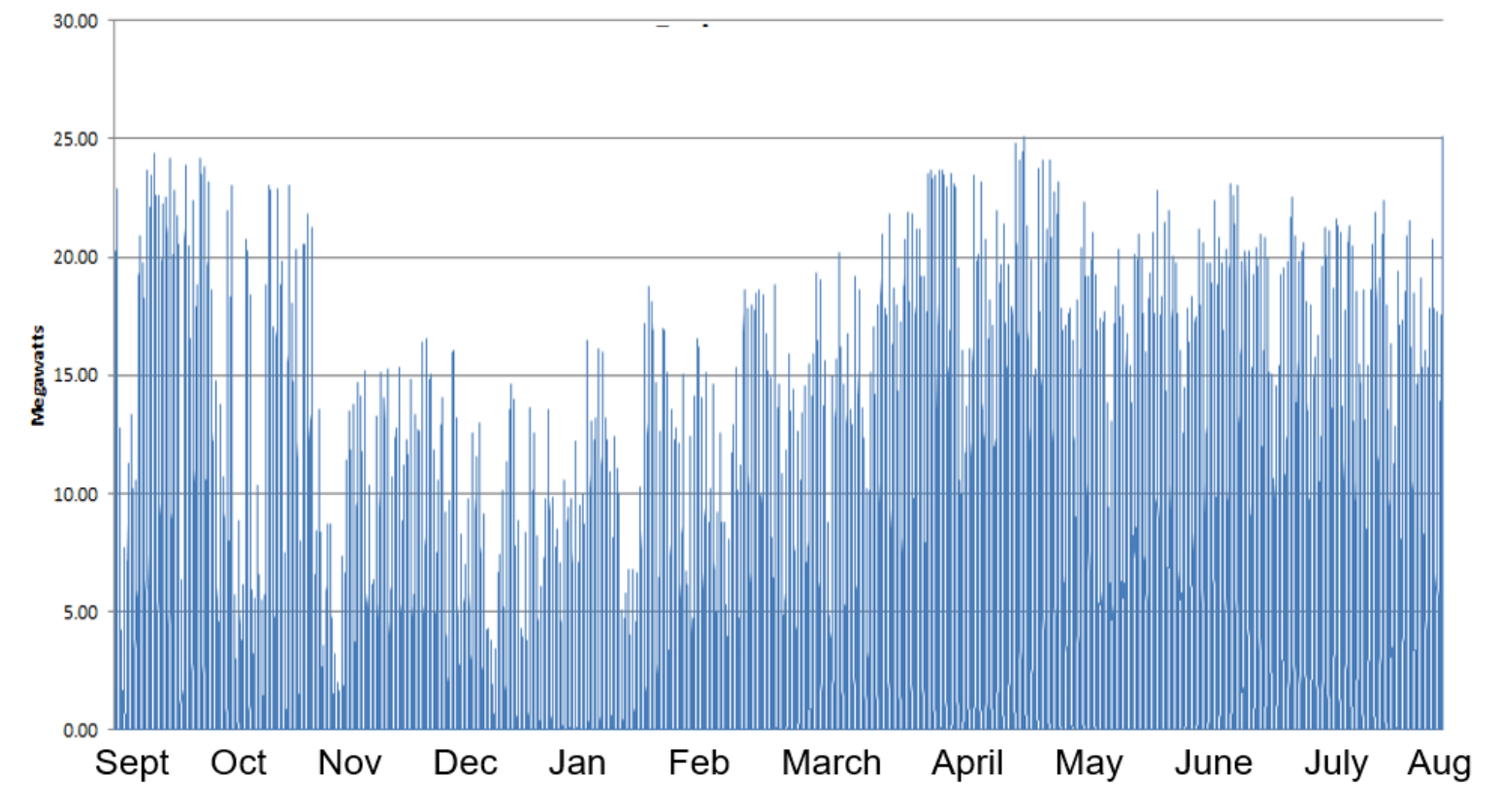
- Fine-grained variability – This might arise at time scales of seconds (even fractions of a second), minutes, hours, or daily. Examples of fine-grained variability are:
- High-frequency trading in finance - These decisions are made several times per second.
- Frequency regulation for the power grid - These are signals sent every two seconds to generators to make adjustments so that the power voltage stays within a narrow range.
- Hourly sales of different restaurant food choices which may require some preparation in advance of service.
- The hourly variations in wind speeds, shown in figure 5.1. This figure would also capture hourly to daily variations in cloud cover, all in the context of predictable seasonal variations.
- Daily sales of a retail product.
- Daily to weekly variations in hospital admissions with the flu.
- Shifts – The fine-grained variability of a process typically represents variations around a mean, but there are times when the mean will shift. Examples are:
- The random demands for a retail product may shift as a result of a change in pricing for either the product, or a competitive product.
- The rate of hospital admissions for an infectious disease will shift as the disease moves through a population near the hospital.
- The demands for redemptions from a mutual fund, which vary by the minute, will shift when the broader stock market responds to a changing economy.
- The number of people making bids on houses (say, for a given realtor), will shift to different levels as interest rates change.
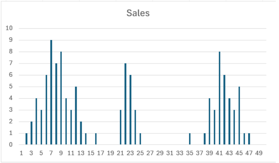
- Bursts, intermittent demands – These describe patterns where there is little or no activity, but then undergoes a burst until it dies down again (see figure 5.2). Examples of bursts include:
- Spread of diseases such as measles – When a disease enters a region, there will be a period of increased infections as the disease moves through the most vulnerable part of the population.
- A product may not be selling, until someone happens to buy it and then spreads the word when they have a good experience. This will spread through their network until it is saturated.
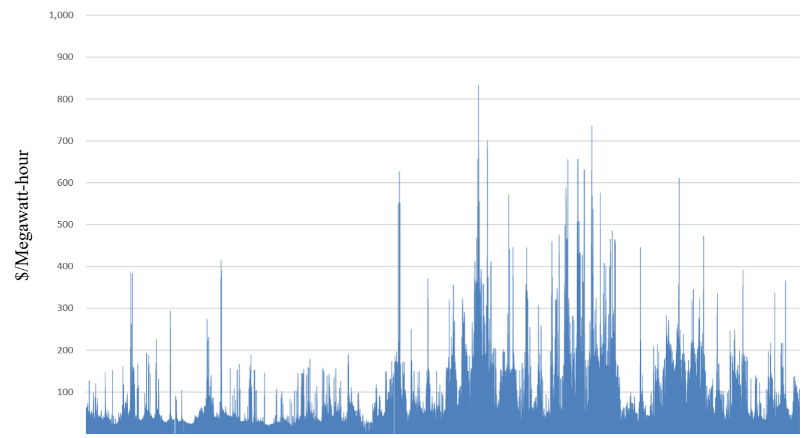
- Spikes – A process may reflect two driving sources. One produces modest outcomes from a well-defined distribution. The second represents infrequent outcomes that are much larger than the first distribution. For example:
- The price of electricity on the grid is updated every 5 minutes. Figure 5.3 shows real-time grid prices for the month of February. It shows a steady sequence of random changes, with occasional spikes that are much larger than the typical variations.
- A storm creates a rush of purchases of milk, eggs and toilet paper.
- A storm system moving past an airport can result in a number of flight cancellations, which in turn can create a large number of last-minute requests for hotel rooms.
- Spatial events (weather, diseases, regulatory) – There are numerous examples of random processes that are regional in nature. Some examples are:
- Weather – Storms can create a range of random events in a region that has been struck by bad weather, or where bad weather is forecast.
- Diseases – Since disease propagation often requires physical contact, outbreaks typically follow a regional pattern.
- Regulations – Changes in regulations typically follow political boundaries, which could be for a country, or a state, district or province within a country.
- Systemic events – These are events that can affect an entire company (spanning international boundaries), an entire country, or even have a global impact, such as:
- Cyberattacks, which can impact information flows for an entire company.
- Public perception – Public events can produce rapid positive or negative perceptions of a company. For example, a beer company undertook a campaign to promote the LGBTQ community, which produced a sudden backlash by their conservative customers which impact sales across the company.
- Rare events – Rare events can arise from a number of sources such as earthquakes, disease outbreaks, or terrorist attacks. These tend to be recognized events that occur quite rarely, but which can have a major impact on an organization when they do happen.
- Contingencies – This category refers to events that might happen, but for which there is no history. For example, grid operators will plan for a failure of nuclear power plants. While this may not have ever happened within a country, the grid operator may still want to prepare for the event if it does happen.
Seasonality
A different form of variability is captured under the general term “seasonality” which comes in various forms:
- Daily cycles – Also known as diurnal cycles, these are all ultimately traced to solar cycles, but these can induce strong daily patterns in human activities. Daily cycles are typically discretized into hours, but finer discretizations (5 minutes, 1 minute) can arise.
- Day of week – This reflects the daily patterns in human behavior set around the different days of the week.
- Hour of week – Hourly patterns may easily depend on the day of week as well as hour of day to capture effects such as Monday morning, Friday afternoon, and daily patterns on weekdays versus weekends.
- Week of month – Manufacturing often has a push to maximize production by month, creating an incentive to push product out before the end of the month. This creates a surge toward the end of the month, followed by a lull.
- Month of year – This captures the familiar seasonal patterns of winter, spring, summer and fall.
- Week of year – Seasonal changes can occur within a month, encouraging the use of week-of-year as a seasonal time increment.
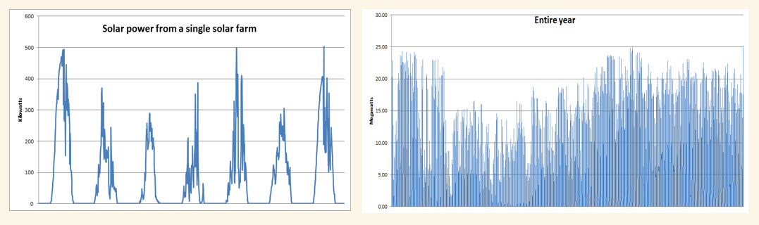
Figure 5.4 (left) shows solar energy production over the course of a week, illustrating both the familiar and highly predictable pattern created by the sun, which is interfered by the highly stochastic presence of cloud cover. Figure 5.4 (right) shows hourly solar energy over the entire year, where we can clearly see the reduction in solar energy during the winter season.
Creating beliefs
If we are modeling uncertainty on the computer, we have to find a way to represent it. Below are several popular strategies.
- Historical data may be used to fit a known probability distribution – There is an entire family of probability distributions we can use to fit to historical data, the best known being the normal distribution. We return to this rich topic later.
-
Use historical data to create a sampled belief model – Imagine we have travel times ranging from 50 to 80 minutes for a trip, depending on the traffic. We can use any of several probability distributions to represent this uncertainty, or we may simply use a sample of past observations, such as:
(52, 63, 78, 59, 71, 68)
-
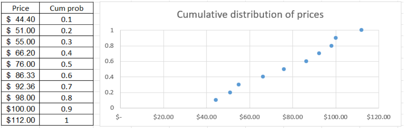
Use historical data to create a quantile distribution from which samples can be drawn – Assume we have a sample of 10 observations of electricity prices, given in figure 5.5 (left). After sorting the prices from smallest to largest, we then show the cumulative probability given in figure 5.5 (right). So, we would say that 60 percent of the observations are $86.33 or lower. These are then plotted in the cumulative distribution on the right.
It is also possible to manually create a cumulative distribution using judgment.
- Use manually created outcomes to represent events that might happen – When we do not have data, we can simply make up possible outcomes. For example, we may be shipping product from Taiwan, which normally takes four weeks. However, we can envision various forms of delays, from hurricanes to backups at the Suez Canal, labor problems at ports or even terrorist attacks. We might feel that we have to allow for the possibility that the shipment might take as long as nine weeks, and then plan for this contingency.
The problem of correlations
The previous section is a brief snapshot of ways of representing the uncertainty in an estimate. However, once we go down the road of recognizing uncertainty, we have to face the far more complex issue of correlations.
It helps to have some examples of information processes in mind to illustrate different forms of correlation. Assume we might be considering any of the following streams of data:
- Customers purchasing a retail product across many sales locations.
- The lead time from placing an order and receiving it.
- The energy generated from a wind farm.
- The rate of new infections from the latest strain of flu.
- The number of truckload movements tendered by a customer to different locations.
These are just a small handful of the types of information streams we will have to deal with. Below we use these examples to talk about three different types of correlations:
- Correlations over time.
- Correlations over geography.
- Correlations over attributes.
Correlations over time
All sequential decision problems involve the element of time, which may be at virtually any time scale, from seconds, minutes, hours, and days to weeks, months and even years.
Correlation over time can arise in each of our five problem settings as follows:
- An incoming snow storm can create a surge in demand for snowblowers; negative publicity can create a period of reduced demand.
- A port strike can create backlogs that increase unloading times for months.
- Rain storms can create periods of increased wind generation that may last for days.
- As a virus enters a region, it will create a period of elevated infections that can last from weeks to months.
- If a plant is shut down for maintenance, there may be a drop in loads out of a location for a week.
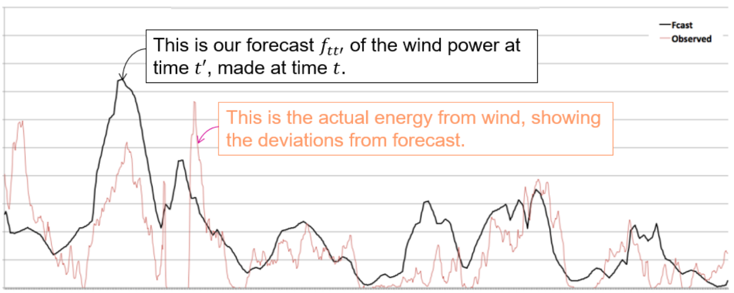
Figure 5.6 illustrates how the energy generated from wind may exceed, or fall below, the forecast over a period of time as weather systems move through a region. It is important that we replicate not just the error between actual and predicted, but also the amount of time we stay above or below the forecast, a quantity known as the “crossing time.”
It is fairly common for random signals to be viewed as variations from a base mean, which is usually treated as a constant which has to be estimated. In reality, the “base mean” may also be varying, but on a different time scale. For example, customers walking into a retail store represent random outcomes on a fine time scale, since the behavior of each customer is independent. But they may be responding to market signals (advertising, word-of-mouth) that is also changing, but more slowly.
Arguably the biggest challenge with correlation over time is that it can occur at multiple time scales, at the same time. Independent events (such as how many people come into a store each hour requesting cough medicine) are quite easy to model. The variations that happen on longer time scales are harder because they create what appear to be correlations across time at smaller time scales.
Correlations across geography
Customer purchase decisions, disease outbreaks, and weather are all examples of random processes that vary geographically. Sometimes political boundaries may limit the correlations, but most of the time it is simply distance that governs the strength of the correlation.
Spatially distributed processes typically occur in very high dimensions (there are a lot of spatial locations!). What simplifies geographical correlations is that it is typically fairly easy to capture. Geography may be a pure function of distance, but it can also reflect geographical boundaries as well as population movement patterns. Fortunately, there are powerful mathematical tools help identify and capture these correlations.
Correlation across geography can arise in each of our five problem settings as follows:
- The surge in demand for snowblowers will also be regional since it is responding to snowstorms (which are regional).
- A port delay can produce reduced supplies in the region served by the port, with higher correlations for points closer to the port.
- Rainstorms are also regional, and will create surges in energy from wind farms in the areas affected by the storm. Similarly, hot spells (which are also regional) will produce periods of low wind.
- The spread of flu will be regional since it passes between people who are close to each other.
- Freight is generated either by changes in a manufacturing plant (which is located at one point) or changes in demand, which may be driven by regional forces.
Correlations across attributes
Most of our examples involve activities that are characterized by a set of attributes:
- Demand for clothing will have correlations between garments with similar style but different colors.
- Products that share common inputs (such as materials for clothing, chips for cars, rare earths for motors) may exhibit similar lead time delays when there is a shortage of the input.
- (No apparent use of correlation across attributes for wind energy.)
- New infections may be correlated across people who share features such as age or medical conditions.
- The flow of truckload movements can be correlated when they are moving common commodities or products.
It is often the case that when we expand all the attributes, we find ourselves with so many combinations that the number of observations for a particular combination of attributes may be quite small, and possibly zero. These problems lend themselves to the use of hierarchical estimation methods, where we create different time series by neglecting one or more attributes, and then using weighted combinations.
Exercises
Review questions
- Name the 12 classes of uncertainty, giving one example of each from any application.
- Name seven forms of uncertainty that can describe random processes, and describe a context that might produce each one.
- What are the ways that uncertainty can impact the performance of a system, and give an example of each.
- Name four forms of seasonality.
- Create a cumulative distribution of wind speeds from the following observations:
(17, 8, 2, 12, 9, 28, 10, 8, 35, 12, 15)
Modeling questions
For each of the questions below, try to find as many forms of uncertainty within each of the classes for the following settings, following the tables given in the section above.
- The inventory planning problem in Chapter 2.
- The furniture demand management problem in Chapter 2.
- Planning clinical trials in Chapter 2.
- Running a presidential election in Chapter 2.
- Supply chain finance in Chapter 2.
- Choose a problem setting of your own, ideally one with some complexity, and identify as many types of uncertainty using the 12 classes as a guide.