Chapter 4: Decisions
This entire book is based on the statement:

It goes without saying that before you can address the problem of identifying the best decisions, you have to know what decisions you are making.
Remember from Chapter 1 that there are two types of “problems”: metric-focused and decision-focused. Examples of each are:
- Metric-focused problems:
- Supply chain management – Minimize inventories, maximize operating margin.
- Electric power grid – Minimize energy generation costs.
- Public health – Minimize deaths.
- Managing a truckload fleet – Maximize net operating revenue per driver per week.
- Managing a hotel - Maximize operating profit.
- Running a presidential campaign - Winning the election.
- Decision-focused problems:
- Supply chain management – How much to order, which supplier to use.
- Demand management – How to price a product, what marketing channels to use.
- Electric power grid – Which generators to schedule for operation, which gas turbines to use.
- Managing diabetes – Which medication to use to control blood sugar, what dosage.
- Mutual fund cash management – How much cash to keep on hand to handle redemptions, what stocks to invest in.
If we start with a metric, our challenge is to identify the decisions that will help us improve the metric. If we start with decisions, then the problem is to design the metric. However, even when we think we know the decisions, we have to be sure that we have not missed any.
There is an extensive mathematical literature on the topic of optimizing decisions, but even these books lack a standard definition of what a decision is. Instead, the books will introduce notation such as decision vector “$x$,” or control “$u$,” or action “$a$,” after which they will give examples and hope that the reader “gets it.” While this works for simple problems, it creates a barrier between the mathematical model and real applications.
For complex applications such as managing supply chains or solving public health problems, identifying decisions is much more challenging than identifying metrics. This is not meant to trivialize the identification of metrics, but the concept of metrics is well understood by both domain experts and modelers alike. When asked what decisions are involved, business executives, medical professionals, engineers and scientists often return blank stares. While the word “decision” is familiar to everyone, it does not appear to be a term that they use in daily problem-solving, while everyone understands “metrics” in one form or another.
Decisions and the English language
It seems as if a good starting point for a chapter on “decisions” would be to offer a definition. It helps to note that standard definitions such as those by Webster will include the usual variety of meanings for a word as it is used in the English language. For example, winning a baseball game is referred to as a “decision.” In this book, we only use “decision” to refer to situations where we have a set of choices, and we have to make the best choice which, of course, implies the identification of performance metrics.
We start by noting that decisions are always a form of information. It helps to put all information into three broad classes:
- Information that we already know at a point in time. We refer to this information as the state of our system (more precisely, the state of knowledge).
- Information that we control that changes the state.
- New information that arrives that we do not control (although we may influence it).
Information in classes (2) and (3) produce an updated state variable (class 1). We are now ready to define a decision:
Definition (formal): A decision is an endogenously controllable information class.
So, decisions (which are contained in “decision variables”) represent information that we create by naming one out of a set of choices.
Our formal definition requires a lot of overhead for what should be a very simple concept, so we offer a second definition:
Definition (informal): A decision is something we control.
This definition avoids “information class” by using “something,” but it gets the point across.
Both our definitions raise the question of who is making the decision, which is inseparable from the concept of a decision. Classical mathematical models avoid this question, but it is central to the modeling of most real systems.
Given the importance of decisions in human activities, it should not be surprising that there are a number of terms in English that capture the concept of a choice. Table 4.1 lists a number of words that imply making a choice in a general setting. Under the column “Collecting information” are terms that arise when deciding what experiment to run, who to listen to, what to observe (and so on). The column labeled “Acting on resources” list a variety of terms that arise in the context of managing resources (such as people). For example “promote” implies the decision of whether or not to promote someone (and to what level).
This table is not intended to be a comprehensive list of words that imply a choice, but it hints that “decisions” come in many ways in the English language.
| General terms | Collecting information | Identification decisions | Acting on resources |
|---|---|---|---|
| Action | Experiment (which?) | Identify | Promote (who, how much) |
| Choice | Listen (to what?) | Classify | Acquire (which, how much) |
| Control | Observe | Finding | Sell (to whom, how much) |
| Decision | Test (which one) | Conclude | Reward (how much) |
| Design | View/scan | Label | Criticize (who, how) |
| Intervention (medical) | Move (to where) | ||
| Option | Trade (which, to whom) | ||
| Move (where) | Treatment (which one) | ||
| Response (which one) | Accept/decline | ||
| Task | Recommend | ||
| Trade (finance) |
Identifying decisions
Understanding all the different words that imply (or require) making a choice is important when identifying the decisions that are available to be made. It is important to recognize that decisions do not come with bright labels attached to them. Campbell’s Soup Co. recognized the challenge of making consumers aware that they were making decisions in a famous series of commercials in the 1970s labeled “I could have had a V8!”. Their marketing department realized that people would often pick up a can of soda without realizing that they could have chosen to have a V8 instead. The commercials helped to make consumers aware that drinking a soda was a decision.
People in almost any problem setting fall into the habit of solving problems a certain way, without realizing that they have choices. One might say that this is how we get through the day, since evaluating choices to identify the best one takes time. The challenge we face is to first be aware of when we are making a decision, and then identifying the decisions that have the biggest impact on performance.
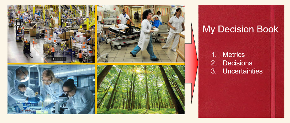
The behavior of passively making decisions is absolutely pervasive, but this creates an opportunity. Imagine that you are in any problem setting (such as those illustrated to the left in figure 4.1). Now assume that you want to improve performance, whether it is profitability, productivity, improved health outcomes, better drugs, or improving agriculture. Then remember our basic line:
If you want to run a better {anything} you have to make better decisions.
To make a better decision, you have to recognize when you are making a decision. A good exercise is to create your “decisions book” and then make mental notes as you recognize when a decision is being made (which is to say, there was a choice, and different choices could be made).
Types of decisions
Our approach to framing requires being able to identify all decisions, not just decisions that can be handled by a particular methodology. To guide this process, we list below 10 types of decisions which, to our knowledge, cover every form of information that we control.
- Physical and financial decisions – These decisions arise in the management of physical and financial resources, spanning people, equipment, facilities, products, commodities, water, energy, in addition to cash, investments, loans, … Decisions include buying, selling, moving, and modifying resources. This class is the domain of operations research, engineering control, and finance, and draws heavily on tools such as linear, integer and nonlinear programming.
- Discrete choices with uncertain outcomes – This is a general term designed to cover activities that may involve complex projects such as launching a new product, submitting a drug to clinical trials, or purchasing a company. Sometimes called “projects,” these may involve a series of changes to performance metrics, resources, finances, and system dynamics. Special cases can be simpler problems, such as picking a price or who to hire for a leadership position. These problems are popular in the decision analysis literature, and typically involve relatively small sets of actions that are difficult to evaluate.
- Information acquisition/observation decisions – These include decisions to acquire or observe information by running experiments in the lab, field, or with computer simulations. It helps to distinguish two settings in which we may acquire information:
- Offline learning - These are activities that are conducted in a test environment. Offline information acquisition can include research efforts, internet searches, or hiring domain experts.
- Online learning - This covers decisions to run and observe processes in the field using a “learning while doing” approach, which involves observing a process as it evolves, such as how a market responds to advertising or pricing, or how a patient responds to a treatment.
Both styles of information acquisition imply making decisions specifically to acquire information. Information acquisition has been studied under names such as design of experiments (static or sequential), stochastic search, active (or optimal) learning, multiarmed bandits, and Bayesian optimization.
- Information communication/sharing decisions – These come in two forms:
- Messaging – This reflects what we say in text, video and/or audio. A modern example of messaging includes prompt optimization.
- Channels and timing – This reflects the choice of channel (text/emails, publication (print or online), social media, or advertising channels) along with the timing and frequency.
- Performance metrics and objectives - These represent the critical choice of quantifying what we are trying to achieve, such as maximizing revenues, minimizing costs, maximizing the strength of a material or performance of a drug, or minimizing empty miles. These can be incorporated into the objective function or represented as constraints.
- Choosing functions – Often overlooked as a decision, functions may be methods to make decisions (policies), the formulation of optimization models, the choice of performance metrics, methods for forecasting or estimation, or transition functions (such as how disease spreads). This category covers the choice of function, which means its structure.
- Setting parameters – Functions are typically characterized by one or more parameters (typically continuous, but not always) that can be tuned to improve predictive accuracy (when fitting statistical models) or optimized to improve performance (when tuning a policy for making decisions). Parameters may be associated with a function; they can be the weight on a performance metric, or they could be a target (or limit) for a performance metric.
- Estimation or identification – We may be given a picture of a person, and asked to identify them, where we want to maximize the number of times we identify the person correctly. A large language model is given a set of words (actually tokens), and it tries to identify the most likely word (or token) that comes next.
- Features and behaviors - We might choose the features of a new software package, the design of a new product, or how we (as an individual, organization or political body) choose to behave.
- Deciding what to decide - In most real applications, the number of potential decisions (that is, anywhere we face a choice) can be quite large. We have to prioritize which decisions have the greatest economic value to justify doing any formal analysis.
Flavors of decision variables
Decisions are going to come in different styles, but decision variables can typically be put in one (or more) of the following categories:
- Binary – Here we have just two choices, which might be:
- To perform an action or not.
- To hold or sell an asset.
- A/B testing for webpage design, where we need to choose between a current design and a new or modified design.
- Whether to continue testing a drug or treatment in a clinical trial, or terminate the trial.
- Discrete set of choices or actions – This is easily the most common form of decision problem, and it arises when we have a set of discrete choices or actions, such as:
- Choosing a supplier for a part.
- Choosing a drug or medical treatment.
- Choosing a marketing channel.
- Choosing a location for a facility.
- Continuous scalar – Examples are:
- Setting the price of a product.
- Choosing the dosage of a drug.
- Deciding how much to spend on advertising in a market for a presidential campaign.
- Choosing how much cash to keep on hand for a mutual fund.
- Discrete vectors – There are many problems that involve the management of discrete resources such as people, machines, and jobs. When we have a single set of discrete choices such as where to purchase a product, it is easy to enumerate all the choices. But when we have to decide how to schedule, say, 100 machines to handle hundreds of jobs, then we need specialized algorithms.
- Continuous vectors – There are problems with a small number of continuous decisions, such as controlling a car, aircraft or rocket. Then there are problems with large numbers of continuous parameters, such as allocating funds across many asset classes, or allocating large numbers of naloxone kits to a hundred counties in a state. There are powerful search algorithms for solving these problems.
How decisions impact the system
It does not make sense to talk about “decisions” as an abstract concept. We first recognize that a decision changes the system in some way, but how?
There are three ways that a decision can impact a system:
- Physical resources – This where we buy, sell or modify in any way anything physical, which could be people, equipment, facilities, food, water, or energy.
- Financial – This can be cash, investments, and loans; insurance contracts, and currency hedges; and prices.
- Informational – This is a category that might include a decision to run an experiment in a lab, computer simulation, or a field test which is used to update estimates or beliefs; it might involve setting performance targets, designing metrics, or specifying the terms of a sales contract.
There is some overlap in the categories, such as the distinction between currency hedges and the terms of a sales contract. What is important is the breadth of ways that we can affect how a system evolves over time.
As we progress in our modeling framework, we are going to need to understand the following about any decision:
- How does the decision affect our performance metrics now?
- What effect will a decision now have on the state of the system before making the next decision?
- Will the decision impact new information that arrives after the decision is made?
In Volume II we describe these points using mathematical notation.
Timing of decisions
One of the most important but challenging attributes of decisions involves time, specifically:
- How frequently decisions are made – We can divide decisions into two broad classes:
- Design decisions, which are made just once (initially) over the planning horizon. In practice, even design decisions evolve over time, but it is common to have decisions that are made just once within what is considered a reasonable planning horizon.
- Control decisions – These are decisions that are made repeatedly over time, but there are complex systems where a variety of decisions are being made at different time intervals. For example, grid operators plan the scheduling of steam generators once each day; gas turbines are planned hourly; adjustments to the speed of certain generators are made every 5 minutes; and signals to adjust the voltage levels are sent every 2 seconds.
- Lag times – When a decision is made, there is often a lag before it impacts the system. For example:
- Ordering inventory may require weeks or months to arrive.
- Administering a drug might take minutes, hours or days before it affects a patient.
- Grid operators plan the schedules for running steam plants the day before, while decisions to turn gas turbines on require 30 minutes notice.
- Pricing changes might not be seen in sales for days or weeks, and may affect markets for months.
- Advance planning of lagged decisions – In addition to the dimensions of when a decision is made and when it impacts the system, we have to think about the timing when we are planning into the future. For example:
- A manufacturer may face lead times of eight months when ordering from Asia, but can get much faster turnarounds for smaller quantities (at higher cost) when there are shortages. When thinking about how much inventory to keep on hand, the manufacturer would have to keep much larger inventories without the option of ordering from the high cost but closer supplier. However when this option is available, the manufacturer can consider the option of using the closer supplier in the event of a surge in demand.
- Airlines often need to plan aircraft purchases up to 10 years into the future, but can negotiate faster deliveries at a higher cost. This allows the airline to consider this as an option if passenger volumes rise faster than planned. Or they can cancel contracts at a cost depending on how long they wait to exercise this option.
Who makes decisions
There are many settings where there is more than one decision-maker (or agent). Examples of multi-agent settings include:
- Two equal decision-makers (often called players) as might happen in negotiations between a manufacturer and a supplier or a customer, or in interactions between a physician and a patient.
- Two decision-makers where one has a controlling position. For example, a “field agent” may ask for resources from a “central agent” who has control over how much of the request to satisfy.
- Several agents, as might arise when a few companies are competing against each other (examples arise in industries that sell cars or industrial chemicals), or when there are multiple organizational units at the same level in a company.
- Multiple agents, as arises in a supply chain with different manufacturers providing components to make a part such as an engine or entire car.
- A single agent learning about an unknown environment, which is how we might model any problem involving uncertainty. The unknown environment could be the weather, the presence of disease in a population, or a market purchasing a product.
We return to multiagent problems later in the series, where we show how to extend the notation (presented in Volume II) to handle multiple decision makers. For now, we are going to focus on a single decision-maker, who may be one of two or more decision-makers.
We have several reasons for avoiding the explicit identification of decision-makers at this stage:
- The organization of decisions can vary, even within the same industry (such as trucking or supply chain management) or problem domain (such as public health).
- If your goal is to develop a computer model, you may be looking to change how decisions are organized. A modeler may wish to treat a set of decisions as if they are being made by a single agent either as a simplification, or because it may produce better results.
- The goal of listing different types of decisions is not to tackle all of them in a single modeling project. Rather, it is necessary to identify the goals of a model and then choose the decisions that are relevant to the goals of the project.
- We recommend that the reader approach these projects from the perspective of a single decision maker, which does not necessarily have to align with how decisions are actually made within an organization. This will be supported by the initial presentation of the universal modeling framework in Volume II.
For now, when faced with a multiagent setting we recommend treating each agent separately to identify their own metrics and decisions. Uncertainties often affect the broader environment, although each agent may have uncertainties that are relevant to their own decisions and performance metrics.
Making decisions with computers
Computers have a very straightforward way of making decisions. It starts by knowing the types of decisions and the set of possible (feasible) decisions. It then uses a prespecified method to “make” the decision, which means a particular choice from the set of feasible (or allowable) decisions.
We start by introducing how we refer to these decision-making methods:
Definition: A policy is a method for choosing an allowable decision using the information that is available at the time the decision is made.
There are two broad strategies for designing policies, each of which can be divided into two classes, creating four classes of policies that include any method for making decisions. These are:
Policy search - This strategy creates functions that have to be tuned to work well over time. They make decisions without directly planning into the future. These can be divided into two classes:
- Policy function approximations, or PFAs.
- Cost function approximations, or CFAs.
Lookahead policies - This strategy tries to make the best decision now by optimizing over the performance of the decision now, plus an approximate of the impact of the decision now on the future. These can also be divided into two classes:
- Policies based on value function approximations, or VFAs.
- Direct lookahead approximations, or DLAs.
Each of these policies is described below.
Policy function approximations (PFAs)
Policy function approximations (PFAs) represent any analytical function which, given inputs from what we know, produces as an output the action we should take. Some examples are:
- Inventory ordering policies often place an order when the inventory falls below a level “s” at which point they place an order to bring the inventory up to “S.” “s” and “S” are parameters that have to be tuned.
- A physician may prescribe insulin injections when a patient’s A1c (which reflects a 3-5 month rolling average of blood sugar) goes above 6.5, and stops when it falls below 6.0. Again, these numbers need to be varied to find the values that work best.
PFAs can be any analytical function such as a linear or nonlinear function. What a PFA cannot include, which will be found in each of the three remaining classes of policies, is an imbedded optimization problem. PFAs can be simple rules, but they can also be very high dimensional nonlinear functions such as a neural network.
Cost function approximations (CFAs)
There are many problems where the best approach for making decisions is to use a deterministic approximation at one point in time which has been modified using various parameters which, when properly tuned, produce decisions that work well over time. This is an approach that is widely used in practice, although often without recognizing a) the ability to introduce parameters to help improve the decisions and/or b) a failure to recognize that the parameters can be tuned to produce better results.
The simplest example of this approach is illustrated in figure 4.2, where we need to choose which product to advertise on social media (we could substitute any problem with discrete choices listed in the intelligent trial and error section of Chapter 2). We have a point estimate for the value of each product based on past experience, which we have learned can involve a lot of noise, resulting in some poor estimates. We can also use past experience to estimate a standard deviation which is a measure of the spread of uncertainty. Typically we are 95 percent sure that the truth is within plus or minus 2 standard deviations.
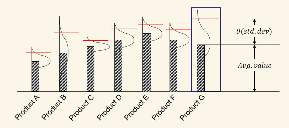
What we are going to do is to create an “index” for each product $x$ given by:
\[Index_x = \text{Avg.value}_x + \theta \,(\text{std.dev}_x)\]We are then going to choose to advertise the product $x$ that has the highest value of “$Index_x$”. We find product $x$ by solving the following optimization problem (which is deterministic):
\[\max_x \{\text{Avg.value}_x + \theta \,(\text{std.dev}_x)\}\]Solving this optimization problem is fairly simple – we just have to sort the values $\text{Avg.value}_x + \theta (\text{std.dev}_x)$ and find the product $x$ that has the highest value (and here you thought deterministic optimization had to be hard!).
The challenge, then, is choosing the tunable parameter $\theta$. If we use $\theta = 0$, then that means we are just using our current estimate. The problem is that if our estimate “$\text{Avg.value}_x$” is low because of a run of bad luck, we might never try advertising product $x$ again. If we use $\theta = 2$, then we are using a very optimistic estimate of the value of product $x$ which will encourage trying products where there is a high level of uncertainty (which is not necessarily a bad strategy).
The idea of using a parameterized deterministic approximation is exceptionally powerful. Airlines use it when they optimize their schedules, where they have to use an estimate of the weather delays for each flight. If they use the median, then half the time the delay will be more than what is anticipated by the schedule, which will then produce a large number of late arrivals of aircraft, delaying subsequent flights. However, if we use the 90th percentile, then we may be introducing too much slack in the schedule, resulting in poor utilization of aircraft.
It is easiest to think of tuning a set of parameters $\theta$ in a simulator, but it is often the case (such as the airline scheduling problem) where the problem is much too complicated. For this reason, it may be necessary to do online learning, which means testing different values in the field and observing the actual performance.
Value function approximations (VFAs)
Imagine that we are dispatching a fleet of trucks where we have to assign drivers to move the loads of freight from a pickup location to a delivery location. Figure 4.3 illustrates how this problem has to be solved repeatedly over time. What we decide to do on Monday will change the locations of drivers on Tuesday and Wednesday. Each day, shippers call in new sets of loads that are not known in advance, so the carrier has to make assignment decisions on Monday without knowing what is going to happen on Tuesday or Wednesday.
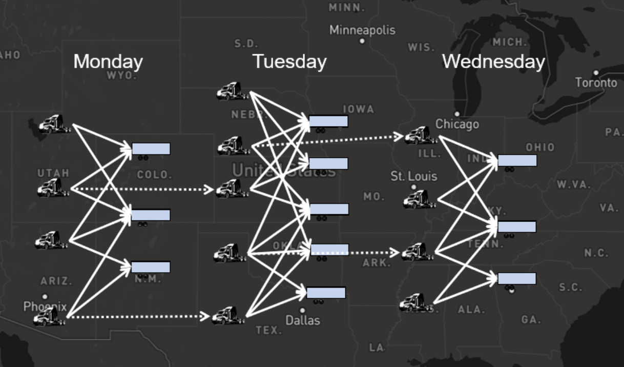
Optimizing over a multiple day horizon in the presence of the uncertainties is an incredibly complex task. Instead, we can approximate the value of drivers in the future, as shown in figure 4.4. This can be done by running simulations into the future, and then calculating the value of drivers in different locations. When we include these values (called “value function approximations”), the problem we now have to solve on Monday is no more complicated than if we completely ignored the impact of sending drivers into different locations.
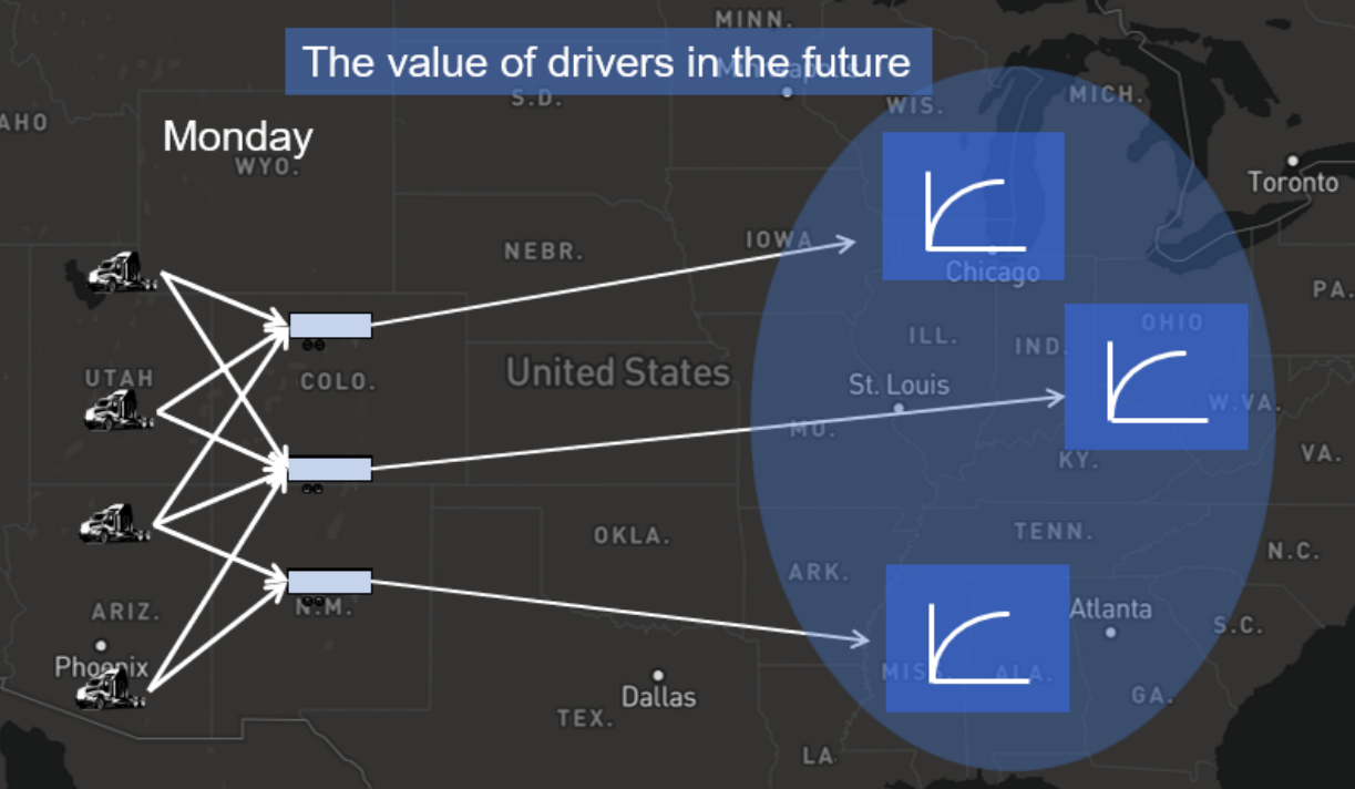
Approximating the value of landing in a particular state is a strategy that is very popular in the research literature, but its success is highly dependent on the structure of a particular problem, and it tends to work well for a small number of specially structured problems.
Direct lookahead approximations (DLAs)
There are many problems where we simply have to plan into the future to make a decision now. One of the most familiar examples of a direct lookahead policy is when we use Google maps to plan a path to the destination.
DLA policies can be divided into two subclasses:
- Deterministic lookaheads – This is where we use point estimates of any uncertain quantities such as traffic delays.
- Stochastic lookaheads – Here we want to explicitly model the uncertainty that we face, such as the potential traffic delays that may arise as we are driving to our destination. It helps to further divide this class into two types:
- Problems with discrete choices - These are problems that are typically solved with decision trees.
- Problems where decisions are vectors - Here we need to use the tools of math programming to search over a multidimensional space.
Note that we do not need to subdivide deterministic lookaheads since, even if the decision in each time period is a scalar, the entire lookahead model requires optimizing over the vector of decisions spanning the time periods over the planning horizon.
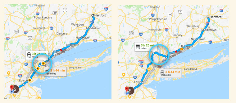
Figure 4.5 (left) shows an example of Google maps planning a path from Hartford, Connecticut (upper right) to Princeton, New Jersey (lower left), departing at 4pm in the afternoon. Note that the path goes right through New York city, which would occur right around 5pm when traffic is expected to be heaviest. Google maps uses a point estimate, and still feels that this is the shortest path.
Of course, any knowledgeable traveler would understand that there is tremendous uncertainty surrounding the actual travel times through New York at 5pm. Figure 4.5 (right) shows an alternate route that Google provides, giving a traveler the opportunity to choose between a path that is expected to be shorter, but with a risk of being much longer, versus a slightly longer path that is expected to be close to the time that Google estimates.
The first path, then, is an example of a deterministic lookahead, but the user can introduce the uncertainty as he assesses the recommendation. By choosing the second path, we are solving, in an admittedly ad hoc way, a stochastic lookahead.
When we are planning into an uncertain future, there is a wide range of strategies for modeling this process to help make a decision now. One strategy is to use a point forecast (that is, a deterministic lookahead) but introduce tunable parameters that can make the solution more robust.
Hybrid policies
In addition to the four classes of policies, we can create a variety of hybrids that combine two, three or even all four of the classes. Some examples using a supply chain setting are:
- CFAs with PFAs - Choosing least cost supplier, but with rules to exclude high-risk companies.
- Lookahead (DLA) with VFA - Optimize seasonal production plan, with functions capturing value of ending inventories.
- Parameterized deterministic direct lookaheads (DLA/CFA) - Plan seasonal production plan using $\theta$-percentile (say, 80th percentile) demand forecasts.
- VFA policy using PFA - Distribution planning using VFAs to value inventory at each warehouse, but using rules (PFAs) to force deliveries to specific locations.
- VFA with CFA - Start with a VFA-based policy with a linear model, and then tune the parameters of the linear VFA to get the best results using a simulator.
While these policies may sound complicated, it is possible to describe specific settings where human decision making is using each of them. For example, the most complex policy uses a stochastic lookahead, which we illustrated above using the navigation problem with Google maps, where a longer path was chosen to avoid the risk of congestion in New York City.
Which policies are most widely used?
Discussing policies can sound complicated and confusing. It is important to remember that:
- Everyone makes decisions. We all face situations on a day-to-day basis, whether to get through the day or decisions that come up in our jobs.
- When we make decisions, our brain is using some method which belongs to one of the four classes (and possibly a hybrid).
Start by dividing the fourth class, DLAs, into two types: deterministic lookaheads and stochastic lookaheads. We are then going to divide the last type, stochastic lookaheads, into two subtypes: problems where decisions are one of a set of discrete choices, and problems where decisions are vectors, such as allocations of assets among investments, or assigning machines to tasks.
This gives us six types of policies that we divide into four categories:
Category 1 - This category includes three types of policies:
- Policy function approximations (PFAs), which include all the simple rules such as “when it is cold, wear a coat” or “buy a product when it goes on sale.” PFAs can be rule-based “if in this state, take this action” or it can be an analytical function, a topic we return to in Volume III.
- Cost function approximations (CFAs), which include any method where we have to solve a deterministic optimization problem (typically an approximation of the real problem that involves uncertainty) such as our discrete choice problem in figure 4.2.
- Deterministic direct lookahead approximations (Det-DLAs), where we plan into the future as is done by Google maps, using point estimates of any uncertain quantity.
CFAs and Det-DLAs both involve solving deterministic optimization problems; the only difference is that CFAs do not plan into the future, while DLAs do.
Category 2 - Stochastic lookahead policies where decisions are discrete choices. Here we explicitly model the uncertainty in the evaluation of each choice. These are widely studied using the device of decision trees.
Category 3 - Policies based on value function approximations, where a decision now considers the immediate cost or reward plus an estimate of the future value from transitioning to some state. This is an advanced and computationally difficult class of policies which are needed for a small set of specialized problems.
Category 4 - Stochastic lookahead policies where decisions are vectors. This is a very complex class of problems that requires complex strategies, since a stochastic lookahead is just another stochastic optimization problem, with simplifications introduced to reduce the computational complexity.
The policies in category 1 are used by everyone, regardless of formal training. These policies are the simplest, but this requires the introduction of parameters that have to be tuned, which can be hard.
Human brains have evolved the natural ability to use all four classes of policies, at least in the context of discrete choices. We even know how to switch between the classes without our realizing it. If we are playing chess (and we have some experience with the game), we probably are doing the first few moves from memory (expert players are able to execute quite a few moves from memory). This is a pure PFA. However, at some point we start to think about what our opponent might do, which involves a direct lookahead policy, typically combined with VFAs which can capture the value of losing major pieces.
Exercises
Review questions
- Give the formal definition of a decision, the informal definition, and three examples of decisions.
- Explain what is meant by an "endogenously controllable information class." What are the other two classes of information that are described in the same context?
- Give examples of decisions that fall in each of the following categories:
- Binary.
- A set of discrete choices with at least five choices.
- There are at least 10,000 different decisions that have to be made at a time.
- Name five examples of continuous decisions.
- Give three examples of each of the three types of decisions:
- Decisions impact physical resources.
- Decisions impact financial resources.
- Decisions impact the collection or distribution of information.
- Name three settings where decisions have to be made at different time scales. Describe the setting and the timing of decisions.
- Summarize in your own words the four classes of policies, and give an example of each for some problem setting.
Modeling questions
- Give an example of a decision that falls in each category:
- A decision that has to be made every minute (or more quickly).
- A decision that has to be made daily.
- A decision that has to be made yearly.
- Identify the decisions implied in each setting, and the decision-maker who makes each decision.
- An individual has to take medication prescribed by their doctor, who is following protocols worked out by the drug developers.
- The power grid has to tell a utility which steam plants to turn on, and when. The scheduling decisions are made by a computer model run the day before.
- A mutual fund manager has to decide how much cash to keep on hand to respond to deposits and redemption requests by individual investors (small amounts) and retail investors (large amounts).
- Give three examples of policy function approximations. Describe the setting and how the PFA would work.
- Give an example of a cost function approximation for a discrete choice problem.
- You are using Google maps to find a path so you arrive at work by 8:30am. You also have to decide how much time to allow so you arrive on time. Describe the decisions being made, and which type of policy is being used to make each one.
- Describe as many classes of policies you might use if you were going to design a computer program to play chess. Describe how each class of policy you have identified would be applied.