Chapter 1: The Fundamentals of Framing
Humanity is comprised of a variety of processes, each of which encompasses a range of activities which can be evaluated in terms of one or more performance metrics. It seems to be a fundamental characteristic that people always want to do better. Athletes want to be faster or stronger; companies want to be more profitable; health professionals want to save more lives; the power grid wants to provide electricity at lower cost.
This book will be defined by the following statement:

We work from the premise that we are always working to improve things, and we can only do so by manipulating elements we control, otherwise known as decisions.
| Application | Objectives |
|---|---|
| Energy systems | Reduce cost, minimize outages |
| Public health | Minimize deaths, maximize productivity |
| Business applications | Maximize profits, minimize costs |
| Supply chain management | Minimize costs, maximize revenue/productivity |
| Manufacturing | Minimize cost, maximize yield, minimize defects |
| Economics | Minimize inflation, maximize growth and employment |
| Finance | Maximize returns, minimize risk |
| Transportation systems (public) | Maximize coverage, minimize cost |
| Freight transportation | Minimize cost, maximize service, meet driver needs |
| Engineering | Maximize strength, minimize cost, maximize performance |
| Drug discovery | Minimize deaths, negative health outcomes, cost |
| Sports | Maximize wins, minimize player payrolls, maximize attendance |
| Entertainment | Maximize views, minimize costs |
Table 1.1 lists a range of human activities, each followed by a short list of metrics that might be used to evaluate performance (the list of metrics can be quite long). These applications hint at the universe of problems where we “want to do better” but the challenge has been creating a step-by-step path that leads to improved performance.
All real-world problem settings need to start with an unstructured, “plain English” description. By contrast, any mathematical model assumes that the problem has already been structured into a form that can be understood by a computer. What is missing is the inputs of people who actually understand the problem, creating the gap depicted by the unfinished bridge that is the front cover of the book.
Standard modeling practice today typically involves someone who is familiar with a “decision technology,” which might be integer or nonlinear programming, or it might be machine learning, or Monte Carlo simulation (today we could throw in large language models which is technically a form of machine learning). When a company reaches out to an expert (whether from industry or academia), they will have an immediate tendency to view the problem from the perspective of their own expertise.
The technical expert will then ask the questions that fit their skill set. The integer programmer will ask about decision variables and a cost function; the machine learner will focus on unknown quantities that have to be estimated or forecasted; the simulation expert may identify design decisions that have to be evaluated using simulation.
This behavior is a form of bias that we call expertise filtering: learning about the problem in a way that reflects their expertise. It happens in virtually every project, since the domain expert will not have the expertise to identify the most appropriate technical expert. The technical experts always assume that their expertise is relevant, and look at problems through the lens of their training. This is not an issue of deception; it is simply human nature.
We take the position that all “problems” are motivated from a desire to improve a process in some way. To improve a process requires making changes which are the result of decisions, and we would like to make better decisions. This perspective seems to turn every problem into an optimization problem since we always want to make the best decisions. This does not mean that we are going to use optimization tools. We do not even presume that we are going to do any formal analysis at all, but we will always keep the door for this open.
We are going to use a much more holistic process toward improving a process. We start by replacing the initial step familiar in the optimization community called “modeling” (translating real problems to mathematical models) with a step we call “framing the problem” which precedes modeling. “Framing” is a well-worn term in business problem solving, but we are going to give it a much more precise meaning.
Our version of framing will be a process that requires training people to ask the right questions which are easier to understand by domain experts (business people, health professionals, scientists, engineers), and which fill in specific elements of a mathematical model if one might be required to solve the problem. Framing should not be done by a technical expert precisely because of the risk of expertise filtering. However, our approach will result in answering questions that would be needed in the use of any analytical tool. We believe that our process of framing will, for many applications, introduce clarity that may help solve the problem even without a computer.
What is a “problem”?
Before we solve a problem, what do we even mean by a “problem”? While there are many varieties of problems, from the perspective of making decisions, we are going to identify two styles:
- Decision-focused problems — These are problems where the decisions we are making are clear:
- Routing trucks
- Ordering inventories
- Pricing a product
- Choosing a medical treatment
- Choosing a battery storage technology
- Locating a facility
- Where to advertise a product, service or candidate
- Choosing which state to visit (running for office)
- Metric-focused problems — These typically arise in more complex situations where we know what we want to achieve, although we may not initially know what decisions can be made to improve the metrics. Some examples of metric-focused settings are:
- Lowering costs, raising revenues or improving profit margins.
- Reducing inventories
- Improving the yield of a manufacturing process
- Reducing infections
- Maximizing financial returns
- Reducing risk
- Improving utilization of people, equipment, and facilities
- Maximizing vote counts (running for office)
Metric-focused problems are generally more complex, since goals are easier to state than the decisions required to achieve a goal. Often we may not even know what decisions might be used to help improve the metrics. Indeed, identifying the decisions that have the biggest impact on the performance metrics is an important step in framing a problem.
At the same time, identifying the right metrics can also be an important step in framing a problem. In fact, in settings with multiple decision-makers (as would happen in any organization), an important type of decision by a manager can be choosing the metrics to evaluate people and business units lower in the organizational hierarchy.
Settings for decision problems
Decision problems can arise in a number of ways:
- We need to make decisions to solve a particular problem at hand that just needs to be solved once.
- We have a well-defined set of decisions, and simply want to do better. In most cases, the decisions are being made by people, and there may be the hope that computers could do better.
- We want to improve our performance over time, especially when we are not meeting expected targets. For these problems, we may not even know in advance what decisions affect performance.
- We have a well-defined set of decisions being made by people, and we would like to automate the process to remove the manual component, possibly as a form of cost reduction (not having to pay for the people), or to gain more control over a process.
- We are simulating decisions for the purpose of planning the system in the future. This could support strategic planning applications, or understanding the impact of decisions made now on the future.
Any of these represent a perfectly sound motivation for identifying a problem to be solved, or an opportunity for improvement. A major challenge is making sure that you are paying attention to the right metrics, and then identifying all the ways you can influence the metrics. Anything that you control falls in the category of a decision.
The three stages of decision automation

An article in the USA Today during the COVID pandemic described the problem of distributing vaccines as “mind-boggingly complex.” The reason for this statement is that people do not know how to think about complex problems. It is sometimes helpful to remember that medieval cathedrals were designed and built by people with no formal education; the problem with vaccine distribution is not the complexity - it is knowing how to think about it.
What has been missing is a structured way for thinking about how to make decisions over time. Our process involves breaking down the process of automating decisions into three stages given by:
Stage I: Framing — Here we identify the core elements of a decision problem which begins by first answering the three questions:
- What are the performance metrics?
- What types of decisions are being made, and who makes them? We make decisions with a method we call the policy.
- What are the sources of uncertainties that affect performance?
Stage II: Modeling — The next step is to fill in the details of the universal modeling process. This starts by answering the following questions:
- How do we make decisions? This is done using a function we call the “policy.” These will be designed from four classes of policies (given in Volume III).
- What information is needed? This makes up the elements of our state variable (alternatively called the “state of knowledge”) which consists of the information required to:
- Make a decision (which depends on the policy).
- Compute any performance metrics.
- Compute (a) and (b) in the future.
Information can be divided between:
- What we know perfectly about quantities of physical and financial resources.
- Parameters and functions used for various purposes.
- What we have to estimate and represent in the form of beliefs.
- How does the state variable evolve over time?
Stage III: Implementation — This ranges from acquiring the information needed to implement and evaluate the decisions. This includes:
- How do we acquire the information that is needed? There is information that is immediately available, information that has to be acquired from other sources, and information that has to be estimated (or forecasted).
- How do we implement the decisions that we make using the policy?
- How do we evaluate how well the decisions perform in the field?
We describe the three stages in the sections that follow.
Stage I: Framing the problem
We refer to the initial stage of the automation process as “framing the problem” which consists of answering the following questions:
- What are the performance metrics?
- What types of decisions are being made (and who makes them)?
- What are the sources of uncertainties that affect the implementation of the decisions and performance of the system?
These three questions are not enough to solve a problem, but they are the starting point for any process that involves making and implementing decisions.
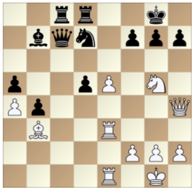
It helps to illustrate these questions for the setting of one of the most challenging games ever invented: playing chess (see figure 1.2). Answering our three framing questions is given by:
- Performance metric – Winning the game.
- Decisions – Allowable moves.
- Uncertainties – Opponent’s moves.
Of course, being trivial to model does not make playing chess easy, but chess was long used as a benchmark for demonstrating the power of algorithmic strategies such as “reinforcement learning.”
Solving the problem arises in Step 4 (Stage II), and while this is quite hard, the remaining steps are also trivial.
Now consider some of the problems that we will identify in Chapter 2:
- How do we reduce deaths due to fentanyl?
- How do we design a supply chain to minimize costs that is robust to different sources of uncertainty?
- How do we manage a fleet of trucks to maximize profits while providing on-time service?
- What is the best strategy for reducing CO2 emissions?
- How should a large manufacturer store and invest its money to maximize returns, while managing risk and meeting short and medium-term cash requirements?
Answering our three framing questions for these problems is a nontrivial exercise. For this reason, we have three chapters dedicated to the process of answering each question:
- Chapter 3 – Performance metrics
- Chapter 4 – Decisions
- Chapter 5 – Uncertainties
These issues are illustrated using the applications in Chapter 2. We provide a brief peek into these three core elements by describing different types of metrics, decisions, and uncertainties in the subsections that follow.
Types of metrics
Metrics come in an endless variety and depend completely on the context.
- Business – Businesses are characterized by long lists of financial metrics, productivity metrics, performance metrics, labor metrics, and metrics capturing how the market is being served.
- Health – Illness/death, cures, side effects, mobility, strength, cost.
- Energy – Cost, quantity of energy provided, outages, demand curtailment.
- Manufacturing - Yield, product performance, speed, cost.
- Drug discovery - Performance, patent protection, market potential, side effects, health risks.
- Sports - Points scored, consistency, fan popularity, injuries, consistency.
- Freight transportation - Revenue, cost, service, labor requirements, exposure to market volatility.
Choosing the right metrics is a challenge of its own, whether you are using them to guide the behavior of a computer model, or to guide the behavior of people.
Separate from what a metric is measuring is how it is being used to guide the performance of the system. Metrics can be used in three different ways:
- Objectives - These are metrics we want to maximize or minimize.
- Targets - We may want the metric to get as close as possible to a target number, such as the temperature in a building or a patient’s blood pressure.
- Limits - We may want a metric to stay under or over some limit. For example, we may want to keep a patient’s blood sugar under a particular value; stockouts should stay under a certain level; financial portfolios need to keep volatility under a specified value.
Types of decisions
An initial list of different types of decisions is given by:
- Binary – These arise when we are choosing between two webpage designs (known as A/B testing), determining when to sell an asset (at each point in time we can hold or sell).
- Discrete choices – It helps to divide this category into three classes:
- A small set of discrete choices - We might need to choose the best drug, the best supplier for a component, or the best location for a facility.
- A set of discretized values of a continuous parameter – Examples are prices, dosages of a drug, or temperatures for baking a semiconductor wafer.
- In some cases the number of discrete choices may be quite large, such as choosing which of 30,000 different molecules that might be used for a drug, or the choice of locations for different facilities spread among 100 different possible locations.
- Continuous choices – Prices, concentrations, dimensions, temperatures, … These can be scalars (that is, a single parameter), or vectors, where we might be optimizing across multiple (potentially many) continuous parameters.
- Vectors of discrete choices – We may have a set of M drivers that we are assigning to N loads, where we have to decide whether to assign driver m to load n.
A second dimension of decisions involves the timing of when a decision made now is implemented in the future. For example:
- A dispatcher assigns a driver to a load to be moved right now.
- A doctor may assign a blood sugar medication that requires several hours to take effect.
- A grid operator will plan today which steam generators should be running tomorrow.
- A supply chain manager places an order that may take several weeks or months to arrive.
- An airline may order new aircraft that may take two years to deliver.
- An investment with a private equity firm may tie up that capital for 8 to 10 years.
A third dimension of decisions involves identifying who makes a decision.
- The management of vaccine distribution involves decisions starting with federal and state agencies, extending through hospitals, physicians and nurses that administer the vaccine.
- The manufacture of automotive engines involves the participation of a sequence of manufacturers who provide the materials, and make the various components of the engine, ultimately moved to market through dealers that control the orders of cars.
- Clinical drug trials involve decisions by scientists, regulators, companies providing the funding, hospitals and clinics that administer the drug, and the patient.
- A trucking company performs dispatching using a team of dispatchers and load managers, which might be replaced with a single computer model that can coordinate these decisions throughout the company.
Forms of uncertainties
Arguably the most subtle aspect of making decisions involves understanding the uncertainties that invariably arise when implementing decisions in the field. Not surprisingly, the forms of uncertainties that arise is heavily dependent on the context. Some examples include:
- Financial trading – Here we are primarily interested in changes in asset prices, but traders are also interested in demand for assets, and changes in other metrics that might suggest where markets are headed such as changes in unemployment, interest rates, retail sales. Markets often move with expectations, which are notoriously hard to measure.
- Supply chain management – Here we have to deal with uncertainties in the market demand for a product, the strategies of competitors, the performance of suppliers, and the behavior of workers (especially when unionized). In addition there are outside influences such as weather, earthquakes and the spread of diseases.
- Public health – The spread of disease is a function of the source of the disease (this may be a single infection, or from many animals who were infected, from which a human strain evolved), the prevalence of the disease, the rate of transmission, how it affects patients, the development of drugs, the distribution of the drugs, and the response of the public in the acceptance of the drugs.
Each of these examples involves multiple sources of uncertainty. These feature different forms of uncertainty, such as:
- Fine-grained noise such as daily random demands.
- Changes in prices and weather typically exhibit spikes and bursts.
- There may be unexpected shifts to new plateaus reflecting shifts in technology, consumer behavior, or competitor decisions.
- Single, rare events such as an earthquake, or invention of a major new technology.
- Contingencies for events that might happen, but which have never actually happened.
The consideration of uncertainty has to be considered in terms of how it affects the performance metrics. When we are making decisions in the presence of uncertainty, we have to make choices, such as how to make a decision, that work well on average given that we do not know what is going to happen in the future.
However, some forms of uncertainty introduce a new dimension called risk that captures factors that are not present in the performance metrics if uncertainty did not exist. Risk is a very popular topic in fields such as finance, supply chain management and health. There are many books that talk about risk, along with very sophisticated papers that model risk, without ever providing a formal definition of risk. We will provide this definition in Chapter 3.
Stage II: Modeling
Our initial three questions (performance metrics, decisions, uncertainties) lay the foundation for what we are going to call our universal modeling framework (or UMF). The UMF can be used to model any decision problem, especially when we use the extended version to handle multiagent problems. For now, we place emphasis on capturing the evolution of decisions and information over time. In Volume II, we will describe the UMF using full mathematical notation (which is not as bad as it sounds), but for now, we are going to sketch it in plain English.
The Universal Modeling Framework consists of five elements:
- State variables capture all the information we need to make decisions and compute our performance metrics. An understanding of the elements of a state variable informs the process of what information is needed to make decisions.
- Decision variables represent what decisions we might make (building on the types of decisions we described when framing the problem). Note that we assume that we make decisions with some “policy” which is to be designed later.
- Exogenous information is any new information that arrives after we make a decision, and before we make our next decision.
- The transition function describes how the state variable changes given what decision we have made, and given the exogenous information that arrived after we made a decision.
- The objective function describes how to evaluate the performance of the system using the method we have chosen for making decisions.
Identifying the state variables requires choosing the method (called the policy) for making decisions, so this has to be done first. However, evaluating and tuning policies requires the entire universal modeling framework if we are going to use a simulator. Ultimately, the design of policies (which plays a major role in determining what information we need in the state variable), and the evaluation of the policies is an iterative process.
The universal modeling framework is covered in much more detail in Volume II where we introduce very basic mathematical notation.
If the universal modeling framework sounds obvious, it is. It is little more than a framework describing the evolution of what we know (the state variable) by decisions (which we control) and the exogenous information (which we do not control). What is perhaps stunning is that this is not standard in the research literature, although there are pockets where it can be found.
Arguably the most difficult step is designing the policy for making decisions. We separate the process of evaluating a policy from designing the policy, which differentiates our approach from that used in virtually every book on stochastic optimization. Fortunately, we have a strategy for overcoming this complexity.
Stage III: Implementation
Easily the most widely overlooked dimension in the design and solution of optimization models is the process of implementing them. The academic literature utterly overlooks that what counts is not how well we solve a problem in the computer, but rather the impact of decisions when they are implemented.
The key dimensions of implementation cover three areas:
- Acquiring the data needed to fill out the state variable, which means the information we need to make decisions and compute the performance metrics (more details are provided in Volume II).
- Implementing the decisions, which might mean getting people to follow instructions, or communicating the instructions electronically.
- Evaluating performance. For complex systems, understanding how well the system is performing, which presumably is affected by the decisions being made, can be quite difficult.
For complex problems in industry, implementation can be an exceptionally challenging process. Even if this is viewed as outside the scope of the modeling process, it helps for modelers to think about these steps. It may be that some decisions are simply never going to be made by a computer. For example, allocating resources in a public health setting involves negotiating between state, regional and local organizations which each have their own hidden priorities.
Three types of information
We first recognize that any quantity that can be represented on a computer is a form of information. We can identify three types of information from the perspective of how it evolves over time:
- The information that we know at the time we make a decision which constitutes the state of our system (more precisely the state of knowledge). This is the information needed to make decisions and/or to compute the performance metrics, now or possibly in the future.
- New information that we control. We define decisions formally in Chapter 4 and describe 10 different types of decisions which helps in the process of identifying decisions.
- New information which arrives from outside of our system beyond our control, although it may be influenced by our current state and/or the decisions we make. We call this exogenous information, and it can come from a number of sources:
- Natural phenomena such as weather and earthquakes.
- Markets, such as the demand for a product, stock prices and interest rates.
- Population dynamics such as the spread of diseases.
- The behavior of other companies or organizations.
- Decisions made by people (more generally, agents) from outside of our system, such as:
- The production decisions of suppliers of inputs to a manufacturing plant.
- Other divisions within a company (such as pricing and marketing, if we are in manufacturing or inventory planning).
- The actions of a patient (if you are the physician).
- Advertisements placed by the competing candidate in a presidential election.
Exogenous information is described in greater depth in Chapter 5.
Decision making as a process
There is a vast literature that focuses on creating “optimization problems” that consist of:
- A decision (or set of decisions).
- An objective to be minimized or maximized.
- Constraints, which determine the set of allowable decisions.
Real decision making is a process, and understanding this process is critical to designing methods for making better decisions. We start by identifying the following elements:
- Sequential decision problems, which describe the process of making a particular set of decisions over time by a single agent.
- The “information chain” which describes the process of creating the information needed to make a decision.
- The steps involved in implementing decisions.
- The process of evaluating performance.
Beyond the scope of this monograph is the challenge of coordinating across multiple decision-makers.
Sequential decision problems
We are now ready to write out, in English, a sequential decision problem, which we can state using:
State, decision, information; state, decision, information; …, state, decision, information.
Each triplet {state, decision, (exogenous) information} represents the information associated with a particular time period:
- “State” is the information we know at the beginning of the time period.
- “Decision” is our endogenously controllable information.
- “(Exogenous) information” is the information that arrives after we make a decision, and before we make the next decision.
After we make a decision (sometimes after we observe the exogenous information) we stop and calculate performance metrics.
Of course, not all decision problems are sequential decision problems, although the vast majority of decisions are made repeatedly over time. However, we can identify several categories of sequential decision problems from the perspective of the sequencing of decisions and information:
- Make decision, stop.
- Make decision, see exogenous information, stop.
- Make decision, see information, make one more decision, stop.
- Make decision, see information, make decision, see information, …, repeat $T$ times, stop.
- Make decision, see information, repeated infinitely.
Some comments:
-
Category 1 describes static, deterministic decision problems that have dominated what is known as the optimization community since the 1950s. The simplest version of these problems might involve finding the best of a set of choices, such as purchasing an item from the least cost supplier, as long as we assume that the item will perform exactly as we expect.
More complex problem instances might involve finding the least cost allocation of supplies from multiple sources to serve different needs, or assigning different people or machines to perform different tasks, introducing the complexity of working in multiple dimensions. The complexity of these problems has led to the astonishing oversight that the vast majority of applications are actually sequential decision problems, a property that has been completely ignored in the literature on this topic.
- Category 2 describes problems known as stochastic search, which represents one of the most widely studied classes of problems. Examples of stochastic search problems include:
- Pick a set of manufacturing facilities and warehouses, and then run a simulation to evaluate its performance.
- Pick a treatment regimen for a patient, and then see how it unfolds.
- Set an investment strategy for a stock portfolio, and then observe how well it works.
All these can be described by “make choice” and then “see how well the choice works.” If this is done in a simulator or a laboratory, we may be able to run these experiments over and over. In this case we have a fully sequential search process that falls in category 4.
- Category 3 describes a more general version of category 2 where we might make an initial decision, such as sending product to a set of warehouses. Next the demands for the product at retail outlets are revealed. Finally, we have the decision of shipping from warehouses to the retail outlets. This problem has been widely studied under the umbrella of stochastic programming.
- Category 4 is the most common form of sequential decision problem since it captures the repeated nature of making decisions followed by learning new information, but we stop after a specific number of time periods, typically for the practical reason that we are running a simulation that has to have a predefined stopping point.
- Category 5 is a popular topic in communities such as dynamic programming (specifically Markov decision processes) and stochastic control. The objective is usually the infinite discounted sum of costs or rewards. This literature typically assumes that the information arriving in each time period comes from the same distribution (this is known as a stationary distribution) and is useful for deriving a variety of theoretical results.
From optimizing decisions to policies
When we are solving a static, deterministic optimization problem, virtually every author represents the decision as a variable (typically a vector) “$x$” where we have to design an algorithm to find the best “$x$.” By contrast, when we have a sequential decision problem, there is a fundamental lack of understanding of what it is we are optimizing over. In a nutshell, with deterministic problems we are looking for the best decision $x$, while for sequential decision problems we are searching for the best function (that is, the policy) which represents a method for making decisions.
The idea of finding the best function for making decisions seems foreign in the optimization literature. By contrast, this is exactly what is done in machine learning, where the challenge is to find a function (often called a statistical model) that does the best job of fitting the data. Moving forward, we will refer to the functions for making decisions as policies, a topic that we address in greater detail in Volume II.
The information chain
Making a decision enjoys certain parallels with making physical products. To make a car (for example), it is necessary to make various parts, which often take multiple steps. Then, after we make the car we have to distribute it to the customer.
Decisions are “made” from information, which itself may need to be created (collected or estimated) through a series of steps. Deciding how many, and what types, of cars to make may require a forecast that is compiled from historical data, as well as economic forecasts and estimates from a sales force. This data then has to go through a set of methods that create the forecasts.
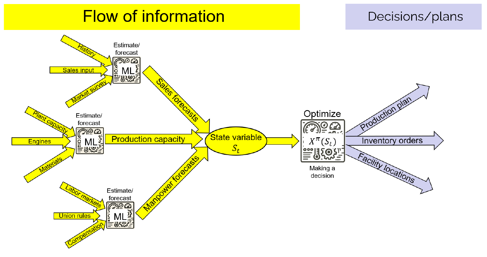
The flow of information is depicted in figure 1.3. “Information” might be observed inventories, a forecast created from history, the result of a decision to collect information through a market survey, or the result of a production planning process. The processing nodes are mathematical functions – sets of equations that act on the inputs to produce an output. The functions may do anything, from adding up numbers to producing forecasts to making decisions by solving an optimization problem.
Just as with physical processes, information processes typically consist of manual steps (such as entering inventories) combined with steps that are done on the computer (and hence are automated), such as running a forecast.
It is easy to think that, given the extensive use of computers, information processes should be almost completely automated. However, there are still a lot of white-collar workers, and they are not loading trucks or working on an assembly line.
Artificial intelligence
Ultimately the goal of thinking about a complex problem in a formal way is to use the power of the computer to improve the process. Most people will immediately suggest using “artificial intelligence” (often referred to as “AI”). The problem is that “AI” is a term that has been used since the 1950s, and has evolved steadily over the years, typically being applied to the latest invention coming out of the field of computer science.
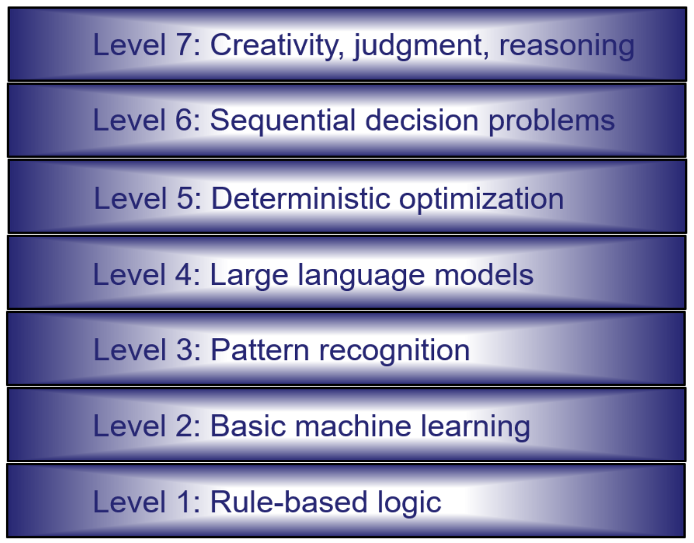
We divide the major forms of AI into seven levels, depicted in figure 1.4. After we describe these seven levels, we will organize them into four fundamentally different classes of intelligence.
The seven levels of AI
Level 1: Rule-based logic - This first evolved in the 1960s and 70s, and emerged in the 1980s (as computers first became much more widely available) as “expert systems.” These consist of rules specified by humans of the form “If {condition} then {action}.” For example, the condition might be “eating red meat” and the action could be “drink red wine.” Or the condition could be the attributes of a patient (symptoms, gender, age, weight, smoker?, blood pressure, …) and the action could be a medical treatment.
This form of AI went through what has become known as the “hype cycle” where people fantasized how computers were going to take over the world.
The problem with rule-based systems is that as the number of elements making up a condition grew, the number of possible condition/action pairs increased exponentially (a behavior known as the “curse of dimensionality”). By the 1990s, this early form of AI was widely viewed as a failure, but in fact rule-based systems remain widely used even today. The only failure is that they did not live up to the initial hype. Rule-based systems are widely used today.
Level 2 – Statistics/machine learning - Under development since the early 1900s, statistics (known as machine learning in computer science) is the science of using data to estimate models. We might use observations of different prices of a hotel room to estimate the demand, or historical demands to forecast the future. This field grew explosively in the 1980s and 1990s (as computers became widely available).
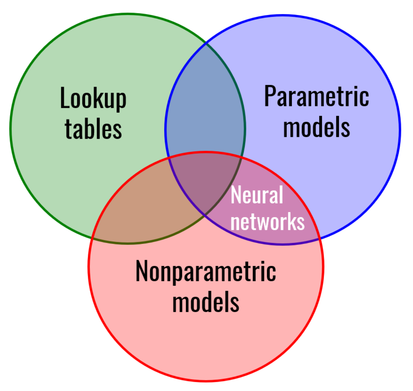
Machine learning models come in a variety of styles, but these can be organized into three broad classes as illustrated in figure 1.5:
- Lookup tables – These are of the form “If {input} then {output},” similar to rule-based systems.
-
Parametric models – These are analytical functions of inputs that produce one or more outputs using a mathematical function that depends on a set of unknown parameters. If the function is linear in these parameters, then this would be a linear model. More general models use functions that are nonlinear in the parameters. Figure 1.6 illustrates linear and nonlinear models.
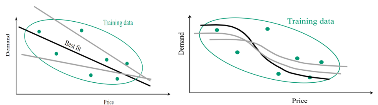
Figure 1.6. Illustrations of linear and nonlinear parametric functions used in machine learning. 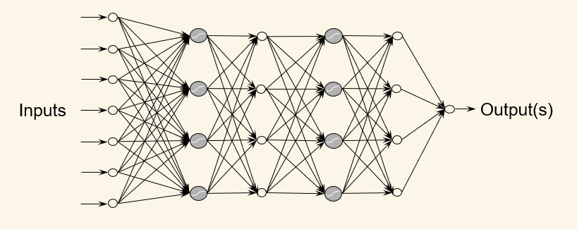
Figure 1.7. Illustration of a (very small) neural network. Each link carries a parameter that has to be tuned so that the output comes as close as possible to the label associated with the inputs in a training dataset. An important class of parametric models which first emerged in the 1970s is neural networks (see figure 1.7). Neural networks have an input layer, where any set of inputs enter the network through the input nodes. These values are then transformed through the intermediate layers before producing one or more outputs. Each link in the network has a parameter associated with it, where the early neural networks often had thousands to a million parameters.
It is best to think of neural networks as a very high-dimensional nonlinear function that can be used to fit a virtually unlimited set of relationships, but at a cost of requiring large training datasets. Also, their flexibility limits their ability to be used in the presence of noise.
- Nonparametric models – These are most easily envisioned as models that are local approximations of a function. For example, we may have estimates of a function at a set of points, and we then use linear extrapolations of these points to provide estimates of points for which we do not have an estimate.
Level 3 – Pattern recognition - The next level of AI emerged from the research community in 2010 addressing the problem of pattern recognition. Pattern recognition is just another form of machine learning that we saw in level 2, which involves using neural networks. However, these neural networks are much larger than the ones used in the 1990s. Instead of many thousands to a million parameters, these neural networks might have 10 to 100 million parameters. These were referred to as “deep neural networks.”
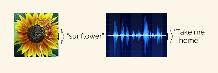
The inputs would be the pixels in an image (or the signals from a voice pattern), which is a much higher dimensional input. The hard part was creating a training dataset large enough to perform the parameter tuning. The training dataset had to consist of millions of images (which was easy to find on the internet) with the associated “labels” which identified the image such as “sunflower” or “Take me home” in figure 1.8. The hard part was getting the labels, which had to be generated by people.
The breakthrough in training came when a Princeton computer science professor, Fei-Fei Li, realized that a software environment created by Amazon called the “Mechanical Turk” made it possible to reach out to people around the world willing to work for very low wages to create these labels. In other words, the breakthrough was not so much the underlying analytics (neural networks were developed back in the 1970s) but rather access to enough data at low cost.
Level 4 – Large language models - Level 4 is simply another step up from image recognition, where instead of estimating (or “predicting”) the identity of an image, the neural network was taking as input a sequence of words (anywhere from a few words to hundreds or thousands of words) to predict the next word (the models act on word fragments known as “tokens”). It does this by creating a probability distribution of the words that might come next given a sequence of words which could be an initial prompt provided by a user.
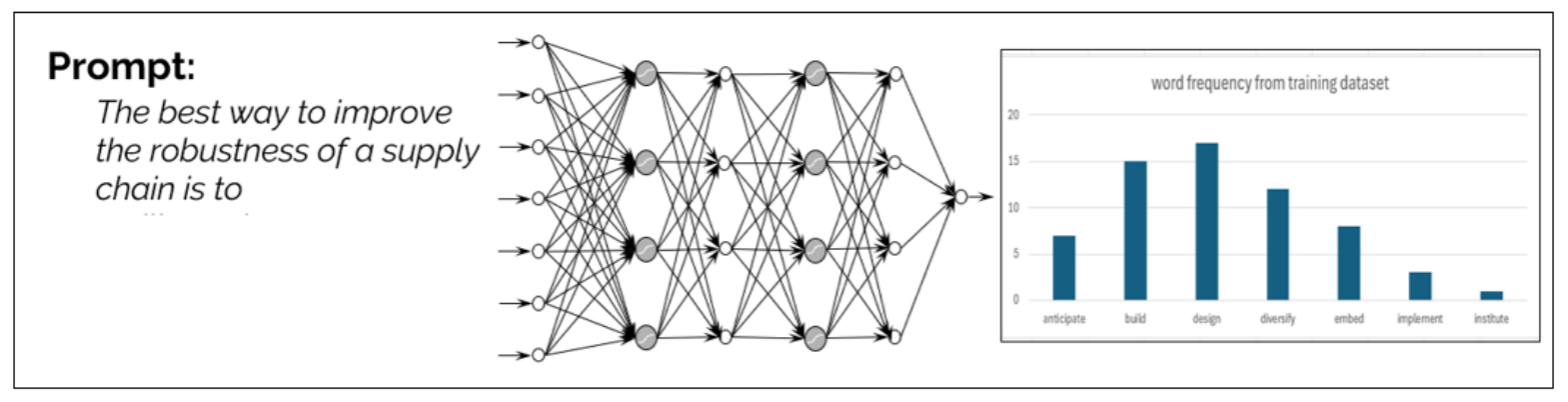
Figure 1.9 illustrates this, starting with the prompt “The best way to improve the robustness of a supply chain is to…” The neural network then produces a probability distribution of the word that might come next, based on the training dataset. The large language model (or LLM) then samples from this distribution, in proportion to the distribution. If it chooses the word “design” then the sequence “The best way to improve the robustness of a supply chain is to design…” is input to the neural network, which then produces another distribution of words. The process of sampling a word, adding it to the previous sequence of words to produce a new sequence, is repeated over and over. This is why the process is called “generative AI.”
The neural networks used to generate the distribution of “next words” that follow a previous sequence are truly colossal. While a deep neural network for pattern recognition (Level 3) might have 10 to 100 million parameters, the neural networks used for LLMs might range between 10 billion and 1 trillion parameters.
It needs to be clear from this description that LLMs are not inherently intelligent; they are just mimicking word patterns from a training dataset. They sound intelligent because they are mimicking word patterns that come from an intelligent source (assuming a human wrote the words).
Level 5 – Deterministic optimization – This covers a substantial library of tools for solving hard decision problems. These problems are known as linear programs, integer programs, and nonlinear programs, and they all have the characteristic that a “decision” is a vector, which means it is a set of different decisions (a very large set). Some examples are:
- We may want to decide how much product to send from a set of 10 distribution centers to 200 warehouses, creating a 2,000-dimensional vector that has to be decided.
- Airlines have to schedule their aircraft and the crews (both pilots and stewarding crews) over extended periods (typically quarterly) to maximize utilization while observing rules for maintaining aircraft along with rules for using people.
- A financial manager may be constantly juggling the allocation of capital among 10,000 different investments, giving us 10,000 buy or sell decisions that are made daily.
Often these problems can be depicted pictorially, as shown on the left in figure 1.10, but there is a standard way of writing them mathematically, often starting with the notation on the right. While this mathematical notation will not be generally familiar, universities produce thousands of students each year who are trained to model problems in this format. Then, there are many computer packages, some available commercially while others are available for free, that can solve even large scale problems efficiently.
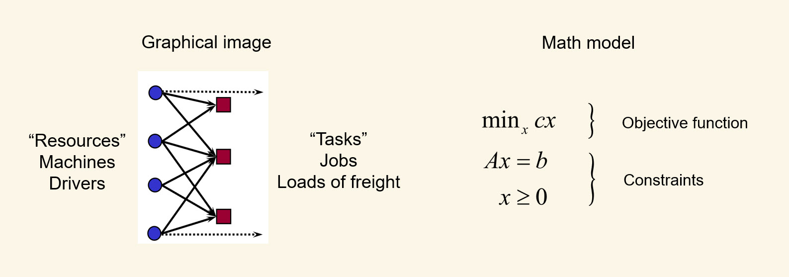
Level 6 – Sequential decision problems – The vast majority of decisions are made repeatedly over time, whether it is every few seconds, minutes or hours, daily, weekly, quarterly or yearly. Even our deterministic optimization problems in level 5 above are usually solved repeatedly over time, but most decisions are much simpler. Some examples of sequential decision problems are:
- Deciding when to sell an asset, and the expected value of holding the asset in the face of dynamically changing prices.
- Replenishing inventory, possibly with very long lead times, to satisfy uncertain demands in a dynamic marketplace.
- Determining the parameters for an automated financial trading policy.
- Choosing the right concentrations of materials, the right temperature for blending and the time to expose the mixture to each temperature to produce a material with the highest strength.
- Choosing the best drug to treat a patient with specific characteristics.
- Deciding how much energy to store from a combination of wind farms, solar farms and the power grid to meet future loads (demands) at least cost.
- Truckload trucking requires determining which drivers to move which loads of freight.
- Choosing how much to invest in each of thousands of stocks and other investments.
Sequential decision problems arise throughout human processes. A decision may be binary (hold or sell), discrete (which drug), or discrete and continuous vectors. Choosing among the best of a discrete (or discretized) set of choices is easily the most common sequential decision problem, but many involve complex operational problems that arise in business logistics, energy systems, and distribution problems in health.
Level 7 – Creativity, reasoning, and judgment – Level 7 represents the highest level of intelligence. For example, while many of the problems in levels 5 and 6 can be quite complex, they always involve well-structured problems with clearly defined decisions and objectives. Level 7 is where we can pose complex problems such as reducing CO2 emissions, minimizing disease, and creating new products.
It is our firm belief that while many authors will talk about the future of “AI” in terms of replacing people, the reality is that computers will not be able to extend past well-defined problems. One activity that we believe is beyond the capability of computer intelligence (including the hyped skills of large language models) is framing complex decision problems. For this reason, we refer to level 7 as science fiction, something that is fun to talk about but will never actually happen.
Three classes of computer intelligence
The first six levels of artificial intelligence represent different forms of intelligence that can be implemented on a computer, while the seventh, in our opinion, remains the sole domain of humans. The first six levels can be divided into three distinct classes:
Class 1 – Human-specified behaviors – This class includes Level 1 in the seven levels of AI, and it can be used for two different purposes:
- Pattern recognition – A rule may specify that if a patient has a specific set of conditions, then it means they have a specific disease.
- Decisions – Similarly, a patient with a specific set of conditions should take a particular medication (which is a form of decision).
Rule-based logic does not distinguish between whether the rule is making a statement about the state of the world, or an action that should be taken. The conditions behind the rule and its outcome (whether it is a statement of the state or a decision) must be manually specified.
An important characteristic of Class 1 artificial intelligence is what it does not use:
- It does not use a training dataset.
- It does not require a model of the underlying decision problem.
Rules have to be directly specified by people, although it is possible for rules to be specified in a dataset. For example, we might have a dataset listing medical protocols, where for each patient condition a treatment is specified. However, imagine we have a dataset compiled of actual physician decisions which may conflict: different physicians may order conflicting treatments despite having patients with identical conditions. If we use this dataset to learn treatments, that would be an example of machine learning.
Class 2 – Machine learning – This class includes Levels 2, 3, and 4. Machine learning refers to the use of mathematical functions that consist of inputs and a set of tunable parameters that can be adjusted so that the function best matches a set of responses, also called labels (among many other names). Machine learning requires a user-specified function, along with a training dataset that consists of inputs and responses (labels).
While rule-based logic is limited in terms of the complexity of the inputs, machine learning can handle very complex inputs using models that have large numbers of parameters. Linear models can have dozens to hundreds of thousands of variables. Neural networks have been trained for large language applications with over a trillion variables. Of course, larger models require large datasets which has proved to be the major barrier limiting the use of neural networks for the highly complex task of language processing.
Class 3 – Optimization – This class includes levels 5 and 6 which address the problem of choosing the best decision from a set of choices, which may be a discrete set or a high-dimensional vector space. Level 5 is limited to static (deterministic) problems where all the data is known, and we seek the best decision (which is often a vector). Level 6 tackles the complex problem of choosing the best decisions over time which spans an absolutely vast range of problems.
The optimization class does not use a training dataset. Instead, it is necessary to specify a performance metric (often called an objective function) along with a set of equations that describe what decisions are allowable. For sequential decision problems, we also need equations that tell us how information evolves over time.
Summary
The methods in class 2, machine learning, aim at training mathematical functions to behave like a training dataset. If the training dataset consists of images such as breast X-rays along with human-generated “labels” of whether the breast displays evidence of cancer, the trained model will never be able to perform any better than the skills of the radiologists who provided the labels. For this reason, it is possible to say that Class 2 methods (machine learning) teach computers to behave like humans (more precisely, behave like the training dataset).
By contrast, the methods in Class 3 (optimization) are designed to produce decisions that outperform humans. The price of this higher-level performance is that we have to provide what is known as a model of the problem. In particular, these methods require a mathematical model, consisting of:
- A well defined set of decisions.
- A clear performance metric that makes it possible to assess whether one decision is better than another.
- The physics of the problem which describe:
- What decisions can be made at a point in time.
- How the system evolves over time.
- How new information is arriving to the system.
This book addresses class 3, since this covers the methods that address making decisions. In particular, we are going to focus on sequential decision problems, since these are the most pervasive – virtually everyone makes decisions, and we make them over time, making them sequential decisions. Static (deterministic) problems are just a special case of sequential decision problems, and the solution of sequential decision problems will draw heavily on the tools developed for static, deterministic problems.
Sequential decision problems represent an incredibly rich problem class. Invariably these tools depend on the methods in the first five levels of artificial intelligence. As with level 5 tools (deterministic optimization), we need a model of the underlying problem. However, since sequential decision problems are much richer than the static problems in level 5, the models need to be much richer and more complex, but this is an area where classical mathematical modeling has fallen short.
Traditional modeling frameworks
It helps to divide the modeling frameworks for making decisions into two broad categories:
- Static, deterministic models that assume that all information is known, where we strive to pick the decisions that work the best.
- Sequential decision models that capture the flow of decisions and information. Since we explicitly model information that arrives after we make a decision, this means that the decisions have to be made before information (presumably relevant to the performance of the decision) has arrived.
In this volume, all sequential decision problems explicitly capture the flow of information, which means that we are making decisions at each point in time before we know the information that may arrive in the future. For this reason, sequential decision problems are fundamentally stochastic (the fancy term for saying the future information is random).
Static, deterministic models
The literature for modeling static, deterministic problems is quite mature, with a substantial base of software built around variations of an optimization model that can be written:
\[\begin{align} \min_{x,y} \quad & C(x,y) \tag{1}\\ \text{subject to:}\\ & g(x,y) = 0, \tag{2}\\ & x \geq 0, \tag{3}\\ & y \in \{0,1\}. \tag{4} \end{align}\]We have allowed for the presence of both continuous variables $x$ (that might take on a value such as 0.56) and discrete variables $y$ that must be 0 or 1.
What happens when modeling deterministic optimization problems (level 5) is that we take the mathematical model given by equations (1)–(4), and we then go to the physical problem and fill in the elements of the model, which requires identifying the decision variables, the objective function, and the constraints. Imagine having a hammer and looking for nails. The tool is useful, but the process requires fitting the problem into the modeling framework.
Deterministic optimization has long emphasized the challenge of designing tools to find the optimal decisions given a model, with secondary attention given to creating the model itself. Note that the modeling framework does not provide any mechanism for capturing the evolution of decisions and information, or anything related to how decisions are organized.
Sequential decision models
Traditionally, the literature for sequential decision problems has tried to follow the same approach, but it has failed completely. In contrast with the well-defined modeling framework for deterministic optimization represented by equations (1)–(4), the optimization literature has not adopted a standard modeling framework for sequential decision problems. As of this writing there are over a dozen different communities using eight different notational systems, with fundamentally different styles for expressing what problem is being solved, or what we are solving for. For example, some communities will write out an objective function as is done in deterministic optimization, others write out a policy, and others will write out an optimality condition.
Our approach depends on the universal modeling framework sketched in the section above, which can be used to model any sequential decision problem. This modeling framework is described in detail in Reinforcement Learning and Stochastic Optimization [chapter 9]. This book lays out the model before describing policies for making decisions, which is done in chapter 11 (chapter 10 focuses on modeling uncertainty).
Volume II of this series will also cover the dimensions of the universal modeling framework in far more detail than we can in this volume, using modest levels of notation. However, the universal modeling framework cannot be used without answering the three questions addressed in this volume.
The most common decision problem
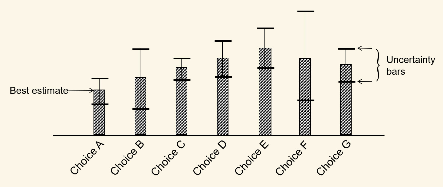
Decision problems, and in particular sequential decision problems, are an exceptionally rich problem class. However, often overlooked in the literature on optimization is that the vast majority of decision problems are described by figure 1.11, where we might have two choices (take an action or not), or a small set of choices (which drug to use, where to purchase a part), or a large number of choices (which product to advertise, which molecule to use when creating a new drug).
A distinguishing characteristic of this problem class is that while we may have an estimate about the performance of each choice, we are typically uncertain about the performance which will emerge after we make a choice. We may just have one chance at making the best choice, but often we make this decision repeatedly, and can learn from past experiences. There are many variations of this problem:
- Whether we are running offline experiments in a lab or simulator, or if we have to learn while doing.
- The number of times we repeat the choice.
- What we learn from one choice may affect our beliefs about other choices, reflecting an underlying belief model.
- The structure of the belief model that captures any underlying structural relationships.
- The presence of physical resources that are being consumed or managed, such as setting up a machine to perform an experiment, consuming supplies, or requiring skilled personnel.
- The time and expense required to make and implement a choice.
The most common approach that people use when choosing from among a discrete set of choices is to simply pick the one that appears to be the best. This ignores the ability to learn from the choice to make a better decision in the future. The value of learning now on future decisions will depend heavily on how many times we will be facing the same set of choices. It may also be ignoring risks that may be associated with making a choice that may perform very poorly.
There are many settings where the decisions are quite important, and we have to live with the decision for a while. Examples might be deciding to develop a particular drug, or choosing a supplier that we have to live with for at least a year. For these problems, it is particularly important to spend some time developing the best set of beliefs about the possible performance of each choice.
Belief models are typically complicated by correlations. Choosing which drug to develop may require comparing different types of cancer drugs that serve a similar market. We may have to choose among a number of suppliers clustered by country which share the same risks of increased tariffs, disease outbreaks, and currency changes.
Static versus sequential decision problems
In the academic literature, there is a strong sense of competition between the community doing deterministic optimization, and the fragmented communities doing optimization under uncertainty. Most deterministic optimization models are deterministic approximations of stochastic problems, and a byproduct is that people using deterministic optimization can be quite defensive when faced with the ways that uncertainty affects their problem.
We urge readers to keep the following in mind:
- A static, deterministic optimization model is just a special case of a sequential decision problem.
- We will show (in Volume II) that deterministic optimization tools are widely used in the solution of general sequential decision problems.
- By far the most common decision problem that arises in practical applications is the one depicted in figure 1.11, where we have to choose the best of a set of choices. Even when we capture the uncertainty in our beliefs about the choices, the different methods for solving this problem still reduce to solving sequences of deterministic optimization problems.
- The problem is not that a deterministic approximation is used; the error is in how the decisions are evaluated. The performance of the decisions have to be evaluated over time as new information arrives.
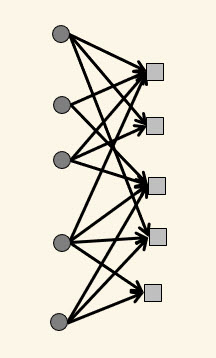
The most common mistake made in the use of deterministic optimization models is to overlook when the problem has to be solved repeatedly over time. An example of this arises in a problem class called an “assignment problem” where we are assigning “resources” (people, trucks, machines) to “tasks” (job assignments, loads to be moved, jobs to be completed). These are never solved just once; as time moves forward, the resources make progress finishing the tasks, new tasks are called in, and the machines may undergo failures changing how long they need to finish a task.
Figure 1.12(a) depicts the problem as a static, deterministic problem. When this problem was first solved by George Dantzig in the 1950s, it was considered a great breakthrough (which it was). However, even 70 years later, top professionals ignore that the problem is never solved just once; it has to be solved repeatedly over time, and it is virtually always the case that the solution at one point in time affects the problems that need to be solved in the (uncertain) future.
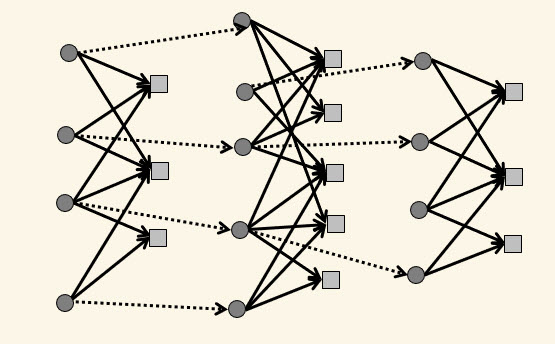
The real problem is depicted in figure 1.12(b), where we illustrate the problem being solved sequentially over time. We note that it is impossible to determine if a deterministic optimization problem needs to be solved sequentially just by looking at the mathematics of the model; it requires understanding the problem in English.
Stages of modeling
We begin by recognizing three different ways of viewing a problem:
- The real world – This is where decisions are implemented, and where we collect information describing the true performance of our system.
- The base model – This is typically in the form of a simulator that is designed to mimic the real world as closely as possible. Simulators (sometimes called “digital twins”) are powerful, but they can be very expensive to develop, which is the reason why we often need to design methods for making decisions without the benefit of a simulator to test the performance of our policy.
- A lookahead model – Lookahead models are used only for making decisions where we have to approximate the impact of a decision made now on the future. Lookahead models are widely used in some form (Google Maps uses an approximate lookahead model to plan a path to the destination), but they are not used universally.
In the discussion of framing the problem above, we described three stages that were involved in understanding the different dimensions of a decision problem. In this section, we are going to focus specifically on developing a computer model, should one be needed.
- Framing the problem: – Any attempt to model a decision problem requires the elements identified in our framing process:
- A plain English narrative – It is important to always start a description in the words of a domain expert with no training in even the process of modeling.
- Answer the three framing questions:
- What are the performance metrics? If you cannot articulate quantifiable performance metrics, you may have one of those complex, unstructured problems that is not amenable to a formal analysis process.
- What types of decisions are being made (and possibly who makes them)? At this point, does simply listing potential decisions make it apparent what choice you should make?
- What are the types of uncertainties that may affect the performance of the system? This can be a complex question that will take time to articulate and then analyze to understand the effect of these uncertainties on the performance of different decisions.
At this point you may feel that the choice you should make is obvious. If not, continue to the next step.
- The universal modeling framework – Understanding the different elements of the universal modeling framework (described above) can provide a more complete understanding of your problem. Specifically:
-
You will need to pull together the information you need to make a decision and compute your performance metrics (also known as the state variables). Since this depends on how you are going to make decisions (the policy), you typically will not be able to identify all the elements of the state variables right away.
Pay attention to information that you would like to have, but cannot observe directly (at least not with any accuracy). These may represent opportunities to use statistical estimation/machine learning.
- Understand what decisions you are allowed to make. Later you will address the problem of making decisions (designing the policy).
- List the types of information that will arrive after you make a decision.
- You will need to think about how your information in the state variable changes over time. Of course, this evolves as our understanding of what information we need. This is the transition function.
- Finally, you will need to understand how you are going to evaluate the performance of your system. This constitutes your objective function.
-
- Modeling uncertainty – This is often the most subtle dimension of modeling a sequential decision problem, often because uncertain quantities may not be immediately obvious. Although there are many potential sources of uncertainty, there are only two ways that it enters the model:
- Uncertainty in quantities and parameters within the state variable, which carries the information needed to make a decision and/or calculate performance metrics.
- Uncertainty in the information that may arrive after a decision is made, but before the next decision is made (we have been calling this the exogenous information process).
There are different ways to capture uncertainty:
- Use observations of uncertain quantities (prices, demands, travel times) from history, and use these samples to calibrate and tune our model.
- Create a mathematical model of the uncertainty, and then generate samples from the mathematical model.
We deal with uncertainty in much greater depth in Chapter 5, where we will identify a number of different sources of uncertainty as a guide to naming the uncertainties that apply to your specific application.
-
Designing policies – Here we address the very rich challenge of designing methods for making decisions. Chapter 4 describes four classes of policies, which capture fundamentally different methods for making decisions, but we defer to Volume III a complete discussion of the process of designing policies.
Note that while we introduce the idea of a state variable in the universal modeling framework, the state variable is partly defined by the information needed by the policy.
- Computer implementation – Once we have designed policies, we have to decide how we are going to test them. The choices are:
- Testing in the field – In this case all we have to do is to implement the policy on a computer, which also means pulling together the data needed to make a decision.
- Computer simulation – How we test policies on the computer depends on the complexity of the system. Typically we are choosing between:
- Spreadsheet implementation – Most problems are relatively simple allowing us to test ideas in a spreadsheet. Spreadsheets can even be the basis of a production system.
- General purpose programming environments – If the problem is too complex for a spreadsheet, we will need to turn to any of a wide range of programming environments. This requires the skills of expert programmers.
- Evaluating and calibrating models and policies – At this point we have to decide if we can develop a simulator to evaluate the policy, or if we need to implement the policy so it can be used in the field:
- Developing a computer-based simulator – At this point we have everything we need to simulate the performance of the policy. A computer simulator is simply a software implementation of the elements in the universal modeling framework. We can then run this simulator either on historical data, or data generated from a mathematical model.
- Field testing – It is often the case that we may not have the time or resources to develop a simulator. Instead, we implement the policy and then monitor how well it works in practice.
Creating a computer-based simulator offers significant advantages, but introduces the difficult dimension of model calibration. By contrast, implementing a policy directly in the field means we are testing it in an environment which requires no calibration. The problem with a field implementation is that searching over different classes of policies, and in particular tuning any parameters, can be painfully slow. Tuning policies in the field has received very little attention in the research literature.
Types of analytics
If we are solving deterministic optimization problems, we can draw on a substantial family of solvers, from commercial packages such as Gurobi or FICO Xpress to any of a wide range of packages that can be downloaded for free. For example, Google offers their “OR Toolbox” at no cost, even for commercial users.
There is very little in the way of commercial tools for optimizing decisions over time as would be necessary in a sequential decision problem. However, we will typically be drawing on several toolboxes as we build custom systems for specific problems. These include:
- Deterministic optimization – Just because we are trying to make decisions over time, under uncertainty, does not mean that the tools of deterministic optimization are no longer used. In fact, most (but not all) sequential decision problems involve solving sequences of optimization problems that are solved using deterministic solvers.
- Simulation – Typically this refers to Monte Carlo simulation which is a body of tools and techniques for estimating functions of random variables. Monte Carlo tools are particularly well suited for high-dimensional, complex problems, making them one of the most powerful tools for modeling the evolution of information.
- Statistical estimation/machine learning – Stat/ML tools, which include linear or nonlinear regression, tree regression, locally parametric models, and neural networks in a variety of sizes. Stat/ML can be described as a set of tools to estimate something we do not know, using information we do know.
These tools are typically described as coming from different communities, of which only one (deterministic optimization) is viewed as solving decision problems. And yet, it is important to understand the role of each for the purpose of making decisions.
Simulation models, for example, are almost always built to help with understanding the behavior of some process, which might be anything from a manufacturing plant to the spread of disease in a population. In both of these examples we are looking to see how the design of the system (the plant layout, where vaccine inventories are held) or the control of the system (how jobs are routed, placing vaccine replenishment orders). We might also simulate the path of hurricanes, and while we cannot change their paths, this information can be used to help guide evacuations which would also have to be simulated.
In short, it helps to think of simulation models as objective functions, or forecasts of future events to be used to make decisions.
So what about statistical estimation/machine learning? While these fields use optimization to fit a model, the goal is simply to estimate a quantity or parameter. But why are we creating these estimates?
We might be estimating the nature of a tumor, or how many people approve of the performance of a president, or the probability a circuit will work. Or we might be estimating events in the future, such as how many people might purchase a product, or the generation of energy in a wind farm. In all these cases, we are creating an estimate or forecast to help make a decision now.
Each of these tools may also provide services with intrinsic value beyond helping to make better decisions. This is most easily seen with the large language models that are rapidly evolving as of this writing. For example, LLMs can help with a growing set of tasks such as doing research, processing requests, and creating images, but not making decisions.
Closing notes
This chapter has laid the foundation for thinking about the complex array of problems known as sequential decision problems. We start from the following premise:
“If you want to run a better {anything} you have to make better decisions.”
The vast majority of settings that involve making decisions fall in the broad category of sequential decision problems, where we make decisions repeatedly over time as new information is arriving (note that a special case of a sequential decision problem is a problem where we just make one decision).
The goal of the volume is building bridges from any problem where there is interest in performing better (presumably by making better decisions), and computer software that can help with those decisions. Computers require mathematical models that capture the problem, and these models need to understand the problem, expressed in English, but using terms that capture the problem in a way that can be translated into the language of models.
A critical feature of this process is the use of a general modeling strategy that we call the universal modeling framework. It is our claim, based on decades of working on a very wide class of problems from many settings, that this modeling framework can capture the features of any problem where computers may be useful. This is an important caveat, since there are problems with poorly defined, or nonexistent, metrics: Whether to marry someone? What field to choose as a major in college? What restaurant to choose when hosting a visitor?
The universal modeling framework formalizes choices such as how to make a decision (called a policy), which then helps answer what information is needed. The UMF also provides a basis for comparing policies which do not need a forecast (buy-low, sell-high in finance, order-up-to inventory policies) against those that do, and to evaluate the value of more accurate forecasts.
Using computers to make decisions opens the door to the use of “artificial intelligence” which is a term that is widely used in the public press without being properly defined. We cover the seven levels of artificial intelligence which clearly differentiate between tools based on machine learning such as large language models (such as ChatGPT), and tools for making decisions such as deterministic optimization (level 5) and sequential decision problems (level 6).
Exercises
Review questions
- What are the three stages of decision automation?
- What are the three questions posed in Stage 1 of framing the problem? Illustrate these in a problem setting of your choosing.
- What are the five elements of the universal modeling framework?
- What is the definition of a decision? Give three examples in different settings that you encounter in your personal activities.
- Briefly describe the seven levels of artificial intelligence, divided into the four different classes as organized in the chapter.
- What are the three classes of statistical models?
- What is the difference between a base model and a lookahead model? Use the context of making a long trip by car using Google Maps to illustrate both of these.
- What are the six stages of modeling?
Modeling questions
- Give an example of a sequential decision problem that you encounter in your daily activities and do the following:
- Identify at least one performance metric that you would like to improve.
- Provide at least one decision that affects the performance metric.
- Describe any uncertainties that might interfere with how the decision performs when it is implemented.
- Give three examples of problems involving physical resources and identify the decisions that arise in each setting.
- You are going to play 15 games of tic-tac-toe where the goal is to force the opposing player to get three in a row (at which point you win). Neither of you have ever played this game before, and you want to capture how the other player learns your strategy of playing. Remember that tic-tac-toe usually ends in a tie, so it will be necessary to get your opponent to believe you are going to make a mistake. Answer the questions below in English (no math allowed).
- Design a performance metric that captures the results of the 15 games.
- What decisions do you have to make?
- What are the uncertainties?
- Describe the information you would have after playing several games that you would want to have to design a policy.